Python实现Logistc回归分类（西瓜数据集、鸢尾花数据集）详解

2023-05-16

文章目录

Logistic回归原理讲解
- 逻辑回归的损失函数
- 梯度下降
代码实现
- 西瓜数据集
- - 全代码
- 鸢尾花（Iris）数据集
- - LogisticModel
  - - 全代码
  - 主函数实现
  - - 全代码

Logistic回归原理讲解

【声明】 笔者实验之前，参考了助教所提供的另一篇文章内容，自行又额外参考一篇CSDN中的相关文章，之后原理讲解将会基于此基础之上进行,引用其中部分内容进行讲解。
Logistic回归（LR）：是一种常用的处理二分类问题的模型，二分类问题中，把结果y分成两个类，正类和负类。因变量y∈{0, 1}，0是负类，1是正类。线性回归函数: f ( x ) = θ t x f(x) = \theta^tx f(x)=θtx的输出值在负无穷到正无穷的范围上，并不好区分是正类还是负类。因此引入非线性变换，把线性回归的输出值压缩到（0, 1）之间，Logistic回归就是通过使用Sigmoid函数，也称为逻辑函数（Logistic function） 进行非线性变换:
g ( z ) = 1 1 + e z g(z) = \frac{1}{1+e^z} g(z)=1+ez1
其函数图像如下：
在这里插入图片描述
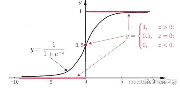
不难看出Sigmoid函数成像为“S形，它的取值在[0, 1]之间，在远离0的地方函数的值会很快接近0或者1，它的这个特性对于解决二分类问题十分重要。将线性回归函数带入Sigmoid函数得到 g ( θ ) = 1 1 + e θ t x g(\theta) = \frac{1}{1+e^ { \theta^tx} } g(θ)=1+eθtx1

逻辑回归的损失函数

通常提到损失函数，我们不得不提到 代价函数（Cost Function） 及目标函数（Object Function）。

损失函数（Loss Function) 直接作用于单个样本，用来表达样本的误差

代价函数（Cost Function) 是整个样本集的平均误差，对所有损失函数值的平均

目标函数（Object Function) 是我们最终要优化的函数，也就是代价函数+正则化函数（经验风险+结构风险）

概况来讲，任何能够衡量模型预测出来的值 h ( θ ) h(\theta) h(θ) 与真实值 y 之间的差异的函数都可以叫做代价函数 C ( θ ) C(\theta) C(θ)如果有多个样本，则可以将所有代价函数的取值求均值，记做 J ( θ ) J(\theta) J(θ) 。在逻辑回归中，最常用的是代价函数是交叉熵(Cross Entropy)函数,此时 J ( θ ) 和 C ( θ ) [ c o s t ( θ ) ] J(\theta)和C(\theta)[cost(\theta)] J(θ)和C(θ)[cost(θ)]如下：
c o s t ( θ ) = { − l o g ( h θ ( x ) ) y = 1 − l o g ( 1 − h θ ( x ) ) y = 0 cost(\theta)=\begin{equation} \left\{ \begin{array}{lr} -log(h_\theta(x))&y =1 \\ -log(1-h_\theta(x))&y=0 \end{array} \right. \end{equation} cost(θ)={−log(hθ(x))−log(1−hθ(x))y=1y=0
J ( θ ) = 1 m ∑ i = 1 m [ − y i l o g ( h θ ( x i ) ) − ( 1 − y i ) l o g ( 1 − h θ ( x i ) ) ] J(\theta) = \frac{1}{m}\sum\limits^m_{i=1}[-y^{i}log(h_\theta(x^i))-(1-y^i)log(1-h_\theta(x^i))] J(θ)=m1i=1∑m[−yilog(hθ(xi))−(1−yi)log(1−hθ(xi))]
有人可能会问为什么log之前要加负号呢？回忆之前提到的Sigmod函数的值域，只落在（0，1）之间，log在此时都为负数，所以负号用于保证值输出为正值。

梯度下降

我们更新迭代参数 θ \theta θ通过梯度下降的办法，通过对 J ( θ ) J(\theta) J(θ)求导，意在不断寻求最小的损失函数值，优化模型
在这里插入图片描述
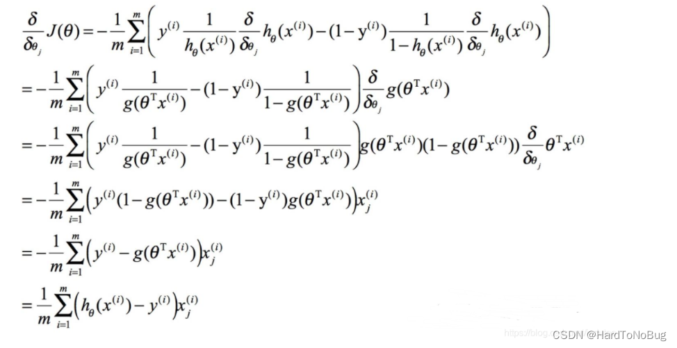
可得到

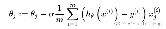
通过不断迭代即可更新学习参数

代码实现

西瓜数据集

实验的第一个部分是要求根据西瓜书上的西瓜数据集进行模型建立。具体其实只给了两个参数，分别是密度和含糖率，所以直接使用Logistic分类模型即可：

density = np.array([0.697, 0.774, 0.634, 0.608, 0.556, 0.403, 0.481, 0.437, 0.666,
                    0.243, 0.245, 0.343, 0.639, 0.657, 0.360, 0.593, 0.719]).reshape(-1, 1)

sugar_rate = np.array([0.460, 0.376, 0.264, 0.318, 0.215, 0.237, 0.149, 0.211, 0.091,
                       0.267, 0.057, 0.099, 0.161, 0.198, 0.370, 0.042, 0.103]).reshape(-1, 1)

在此我们先给出LogistcModel的初步定义：

class LogisticModel:
    def __init__(self, X, Y, alpha=1, mini=0.0001) -> None:
        self.x = X
        self.y = Y
        self.alpha = alpha#学习率
        self.mini = mini#迭代停止最小误差
        cnt = len(x[0])	#样本数量
        self.theta = np.array([[0.0] for i in range(cnt)])
        self.predict = [] #存放预测值

随后就是Sigmoid函数和损失函数的实现：

	def __sigmoid(x):
        return 1/(1 + np.exp(-x))

    def __loss(self, theta):
        # 计算损失值
        sum = 0.0
        for i in range(len(self.y)):
            if y[i][0] == 1:
                sum += - \
                    float(log(LogisticModel.__sigmoid(np.dot(x[i], theta))))
            else:
                sum += - \
                    float(log(1-LogisticModel.__sigmoid(np.dot(x[i], theta))))

        return sum/len(self.y)

之后是编写梯度计算与循环检查函数：

    def __gradient(self, theta):
        # 求取梯度
        sum = 0
        for i in range(len(self.y)):
            sum += (LogisticModel.__sigmoid(
                float(np.dot(x[i], theta))) - y[i][0]) * x[i]
        sum /= len(self.y)
        ans = self.alpha*sum.reshape(-1, 1)
       	return ans
       	
    def __check(self):
        # 检查是否达到迭代边界条件
        TempOld = LogisticModel.__loss(self, self.theta)
        Theta = LogisticModel.__gradient(self, self.theta)
        self.theta -= Theta  # 更新theta
        TempNew = LogisticModel.__loss(self, self.theta)
        result = abs((abs(TempNew)-abs(TempOld)))
        if result <= self.mini:
            return False
        return True

    def fit(self):
        # 迭代梯度下降的过程
        while(LogisticModel.__check(self)):
            pass

最后的步骤就是对模型的预测与结果的输出，这里输出采用的是混淆矩阵（Confusion Matrix）

    def predictSelf(self):
        # 模型预测
        for i in range(len(self.y)):
            if(LogisticModel.__sigmoid(np.dot(self.x[i], self.theta)) > 0.5):
                self.predict.append(1)
            else:
                self.predict.append(0)

    def show(self, labels_name):
        cm = (confusion_matrix(self.y.reshape(1, -1)[0], self.predict))
        # 展示模型结果
        print("accuracy:{:.2%}".format((cm[0][0]+cm[1][1])/(len(self.y))))
        print("presicion:{:.2%}".format(cm[0][0]/(cm[0][0]+cm[0][1])))
        print("recall:{:.2%}".format(cm[0][0]/(cm[0][0]+cm[1][0])))

        cm = cm.astype('float') / cm.sum(axis=1)[:, np.newaxis]    # 归一化
        plt.imshow(cm, interpolation='nearest')    # 在特定的窗口上显示图像
        plt.title('WaterMelon')    # 图像标题
        plt.colorbar()
        num_local = np.array(range(len(labels_name)))
        plt.xticks(num_local, labels_name, rotation=90)    # 将标签印在x轴坐标上
        plt.yticks(num_local, labels_name)    # 将标签印在y轴坐标上
        plt.ylabel('True label')
        plt.xlabel('Predicted label')
        plt.show()

在这里插入图片描述

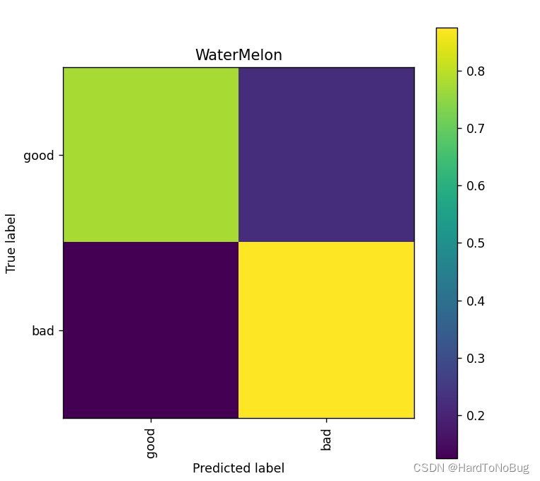
accuracy:82.35%
presicion:77.78%
recall:87.50%

全代码

这里额外解释一下，主函数中的x我是将Sugar_rate与density 合并在一起，y中记录的是真实值的数据。而C起初我是打算用作线性的函数常数项，但是随后发现引入C的准确率并不是很高，各位可以自己下去自行添加尝试。

import numpy as np
from numpy import log
from sklearn.metrics import confusion_matrix
import matplotlib.pyplot as plt
np.set_printoptions(suppress=True)  # 取消科学计数法输出


class LogisticModel:
    def __init__(self, X, Y, alpha=1, mini=0.0001) -> None:
        self.x = X
        self.y = Y
        self.alpha = alpha
        self.mini = mini
        cnt = len(x[0])
        self.theta = np.array([[0.0] for i in range(cnt)])
        self.predict = []

    def __sigmoid(x):
        return 1/(1 + np.exp(-x))

    def __loss(self, theta):
        # 计算损失值
        sum = 0.0
        for i in range(len(self.y)):
            if y[i][0] == 1:
                sum += - \
                    float(log(LogisticModel.__sigmoid(np.dot(x[i], theta))))
            else:
                sum += - \
                    float(log(1-LogisticModel.__sigmoid(np.dot(x[i], theta))))

        return sum/len(self.y)

    def __gradient(self, theta):
        # 求取梯度
        sum = 0
        for i in range(len(self.y)):
            sum += (LogisticModel.__sigmoid(
                float(np.dot(x[i], theta))) - y[i][0]) * x[i]
        sum /= len(self.y)
        ans = self.alpha*sum.reshape(-1, 1)
        # print(theta - ans)
        return ans

    def __check(self):
        # 检查是否达到迭代边界条件
        TempOld = LogisticModel.__loss(self, self.theta)
        Theta = LogisticModel.__gradient(self, self.theta)
        self.theta -= Theta  # 更新theta
        TempNew = LogisticModel.__loss(self, self.theta)
        result = abs((abs(TempNew)-abs(TempOld)))
        if result <= self.mini:
            return False
        return True

    def fit(self):
        # 迭代梯度下降的过程
        while(LogisticModel.__check(self)):
            pass

    def predictSelf(self):
        # 模型预测
        for i in range(len(self.y)):
            if(LogisticModel.__sigmoid(np.dot(self.x[i], self.theta)) > 0.5):
                self.predict.append(1)
            else:
                self.predict.append(0)

    def show(self, labels_name):
        cm = (confusion_matrix(self.y.reshape(1, -1)[0], self.predict))
        # 展示模型结果
        print("accuracy:{:.2%}".format((cm[0][0]+cm[1][1])/(len(self.y))))
        print("presicion:{:.2%}".format(cm[0][0]/(cm[0][0]+cm[0][1])))
        print("recall:{:.2%}".format(cm[0][0]/(cm[0][0]+cm[1][0])))

        cm = cm.astype('float') / cm.sum(axis=1)[:, np.newaxis]    # 归一化
        plt.imshow(cm, interpolation='nearest')    # 在特定的窗口上显示图像
        plt.title('WaterMelon')    # 图像标题
        plt.colorbar()
        num_local = np.array(range(len(labels_name)))
        plt.xticks(num_local, labels_name, rotation=90)    # 将标签印在x轴坐标上
        plt.yticks(num_local, labels_name)    # 将标签印在y轴坐标上
        plt.ylabel('True label')
        plt.xlabel('Predicted label')
        plt.show()


density = np.array([0.697, 0.774, 0.634, 0.608, 0.556, 0.403, 0.481, 0.437, 0.666,
                    0.243, 0.245, 0.343, 0.639, 0.657, 0.360, 0.593, 0.719]).reshape(-1, 1)

sugar_rate = np.array([0.460, 0.376, 0.264, 0.318, 0.215, 0.237, 0.149, 0.211, 0.091,
                       0.267, 0.057, 0.099, 0.161, 0.198, 0.370, 0.042, 0.103]).reshape(-1, 1)
# 用于迭代Theta的常数项
C = np.array([1, 1, 1, 1, 1, 1, 1, 1, 1, 1, 1,
              1, 1, 1, 1, 1, 1]).reshape(-1, 1)
#x = np.hstack((density, sugar_rate),C)
x = np.hstack((density, sugar_rate))
y = np.array([1, 1, 1, 1, 1, 1, 1, 1, 0, 0, 0,
              0, 0, 0, 0, 0, 0]).reshape(-1, 1)
Test = LogisticModel(x, y)
Test.fit()
Test.predictSelf()
labels_name = ["good", "bad"]
Test.show(labels_name)

鸢尾花（Iris）数据集

鸢尾花数据集是一个多分类的数据集，获取方法可以看这篇文章
对于多分类的样本，显然不能直接使用Logistic模型对齐分类，这里介绍一种可以将二分类模型用于进行多分类的方法——投票法（VotingClassifier），以鸢尾花数据集为例，总共提供了3种不同类型的花，那么我们可以将之两两组合，形成3个分类器，预测时三个分类器分别预测其种类对其投票，票数多的即为预测结果，如果票数一致则可以任选一个种类记录：

LogisticModel

我的思路是首先对于之前的模型进行改造，使之可以适应鸢尾花的分类，
主要改变的其实就是画图的部分,去除了计算召回率和精确率（因为要分别对3个分类器求，过于繁杂），其次就是把title和混淆矩阵转移到函数外计算，

    def show(cm, labels_name, title):
        print("accuracy:{:.2%}".format(
            (cm[0][0]+cm[1][1]+cm[2][2])/(np.sum(cm))))
        cm = cm.astype('float') / cm.sum(axis=1)[:, np.newaxis]    # 归一化
        plt.imshow(cm, interpolation='nearest')    # 在特定的窗口上显示图像
        plt.title(title)    # 图像标题
        plt.colorbar()
        num_local = np.array(range(len(labels_name)))
        plt.xticks(num_local, labels_name, rotation=90)    # 将标签印在x轴坐标上
        plt.yticks(num_local, labels_name)    # 将标签印在y轴坐标上
        plt.ylabel('True label')
        plt.xlabel('Predicted label')
        plt.show()

还有就是对于梯度下降的界定条件由0.0001降低了一个百分比到0.001，原因是之后在我计算时，发现对于其中的一个模型来说，原先的精度会需要迭代更多的次数，有可能是深陷局部最小值难以跳出，加之降低精度后最终预测结果也可以接受，故改之。其实也可以改良梯度下降算法，例如：动量梯度下降法（gradient descent with momentum）大家可以自行尝试

class LogisticModel:
    def __init__(self, X, Y, alpha=1, mini=0.001) -> None:
        self.x = X
        self.y = Y
        self.alpha = alpha
        self.mini = mini
        cnt = len(self.x[0])
        self.theta = np.array([[0.0] for i in range(cnt)])
        self.predict = []

全代码

import numpy as np
from numpy import log
import matplotlib.pyplot as plt
np.set_printoptions(suppress=True)  # 取消科学计数法输出


class LogisticModel:
    def __init__(self, X, Y, alpha=1, mini=0.001) -> None:
        self.x = X
        self.y = Y
        self.alpha = alpha
        self.mini = mini
        cnt = len(self.x[0])
        self.theta = np.array([[0.0] for i in range(cnt)])
        self.predict = []

    def sigmoid(x):
        return 1/(1 + np.exp(-x))

    def __loss(self, theta):
        # 计算损失值
        sum = 0.0
        for i in range(len(self.y)):
            if self.y[i][0] == 1:
                sum += - \
                    float(log(LogisticModel.sigmoid(
                        np.dot(self.x[i], theta))))
            else:
                sum += - \
                    float(
                        log(1-LogisticModel.sigmoid(np.dot(self.x[i], theta))))

        return sum/len(self.y)

    def __gradient(self, theta):
        # 求取梯度
        sum = 0
        for i in range(len(self.y)):
            sum += (LogisticModel.sigmoid(
                float(np.dot(self.x[i], theta))) - self.y[i][0]) * self.x[i]
        sum /= len(self.y)
        ans = self.alpha*sum.reshape(-1, 1)
        # print(theta - ans)
        return ans

    def __check(self):
        # 检查是否达到迭代边界条件
        TempOld = LogisticModel.__loss(self, self.theta)
        Theta = LogisticModel.__gradient(self, self.theta)
        self.theta -= Theta  # 更新theta
        TempNew = LogisticModel.__loss(self, self.theta)
        result = abs((abs(TempNew)-abs(TempOld)))
        if result <= self.mini:
            return False
        return True

    def fit(self):
        # 迭代梯度下降的过程
        while(LogisticModel.__check(self)):
            pass

    def predictSelf(self):
        # 模型预测
        for i in range(len(self.y)):
            if(LogisticModel.sigmoid(np.dot(self.x[i], self.theta)) > 0.5):
                self.predict.append(1)
            else:
                self.predict.append(0)

    # def show_theta(self):
    #     print(self.theta)

    def show(cm, labels_name, title):
        print("accuracy:{:.2%}".format(
            (cm[0][0]+cm[1][1]+cm[2][2])/(np.sum(cm))))
        cm = cm.astype('float') / cm.sum(axis=1)[:, np.newaxis]    # 归一化
        plt.imshow(cm, interpolation='nearest')    # 在特定的窗口上显示图像
        plt.title(title)    # 图像标题
        plt.colorbar()
        num_local = np.array(range(len(labels_name)))
        plt.xticks(num_local, labels_name, rotation=90)    # 将标签印在x轴坐标上
        plt.yticks(num_local, labels_name)    # 将标签印在y轴坐标上
        plt.ylabel('True label')
        plt.xlabel('Predicted label')
        plt.show()

主函数实现

首先就是数据的读取和分类器的构建，这里我提供的标签训练值统一为前50位为1，后50位为0的列表，这是为了能够直接复用ModelLogistic类，回忆西瓜数据集时，我们正例标记为1，负例标记为0。这里相当于组合的前50类别标记为正，后50标记为负，因为鸢尾花的数据集十分规整，所以我们可以很轻易地将其分出3个类别。

Labels_name = ['SepalLength', 'SepalWidth',
               'PetalLength', 'PetalWidth', 'Species']
# 读取表格数据
iris = pd.read_csv("D:\Code\python\Iris.csv", header=0, names=Labels_name)
x = np.hstack((np.array(iris[u'SepalLength']).reshape(-1, 1), 
               np.array(iris[u'SepalWidth']).reshape(-1, 1),
               np.array(iris[u'PetalLength']).reshape(-1, 1),
               np.array(iris[u'PetalWidth']).reshape(-1, 1)))

Y = np.hstack([[1]*50, [0]*50]).reshape(-1, 1)
x_SVer = np.vstack([x[0:50], x[50:100]])
x_VerVir = np.vstack([x[50:100], x[100:150]])
x_VirS = np.vstack([x[100:150], x[0:50]])

ModelA = LogisticModel(x_SVer, Y)
ModelB = LogisticModel(x_VerVir, Y)
ModelC = LogisticModel(x_VirS, Y)

ModelA.fit()
ModelB.fit()
ModelC.fit()

随后是编写投票器预测模型，免不了大量if语句：

def predict(a, b, c, test, pre):
    for i in range(len(test)):
        # 记票器
        list = [0, 0, 0]
        if(LogisticModel.sigmoid(np.dot(test[i], a.theta))) > 0.5:
            list[0] += 1
        else:
            list[1] += 1
        if(LogisticModel.sigmoid(np.dot(test[i], b.theta))) > 0.5:
            list[1] += 1
        else:
            list[2] += 1
        if(LogisticModel.sigmoid(np.dot(test[i], c.theta))) > 0.5:
            list[2] += 1
        else:
            list[0] += 1
        if(list[0] ^ list[1] ^ list[2] == 1):
            pre.append("Iris-versicolor")
        else:
            if(list.index(2) == 0):
                pre.append("Iris-setosa")
            elif(list.index(2) == 1):
                pre.append("Iris-versicolor")
            elif(list.index(2) == 2):
                pre.append("Iris-virginica")

这里的测试集需要我们自己划分，调用sklearn中的 train_test_split函数进行划分：

from sklearn.model_selection import train_test_split
y = np.array(iris[u'Species']).reshape(-1, 1)  # 标签
x_train, x_test, y_train, y_test = train_test_split(
    x, y, test_size=0.6)  # 划分数据集

最后一步，预测+输出最终结果：

pre = []  # 存储预测结果
predict(ModelA, ModelB, ModelC, x_test, pre)
cm = (confusion_matrix(y_test, np.array(pre).reshape(-1, 1)))
print(cm)
title = "Iris Prediction"
LogisticModel.show(cm, ['setosa', 'versicolor', 'virginica'], title)

全代码

from LogisticModel import LogisticModel
import pandas as pd
import numpy as np
from sklearn.metrics import confusion_matrix
from sklearn.model_selection import train_test_split
np.set_printoptions(suppress=True)  # 取消科学计数法输出


def predict(a, b, c, test, pre):
    for i in range(len(test)):
        # 记票器
        list = [0, 0, 0]
        if(LogisticModel.sigmoid(np.dot(test[i], a.theta))) > 0.5:
            list[0] += 1
        else:
            list[1] += 1
        if(LogisticModel.sigmoid(np.dot(test[i], b.theta))) > 0.5:
            list[1] += 1
        else:
            list[2] += 1
        if(LogisticModel.sigmoid(np.dot(test[i], c.theta))) > 0.5:
            list[2] += 1
        else:
            list[0] += 1
        if(list[0] ^ list[1] ^ list[2] == 1):
            pre.append("Iris-versicolor")
        else:
            if(list.index(2) == 0):
                pre.append("Iris-setosa")
            elif(list.index(2) == 1):
                pre.append("Iris-versicolor")
            elif(list.index(2) == 2):
                pre.append("Iris-virginica")


Labels_name = ['SepalLength', 'SepalWidth',
               'PetalLength', 'PetalWidth', 'Species']
# 读取表格数据
iris = pd.read_csv("D:\Code\python\Iris.csv", header=0, names=Labels_name)
x = np.hstack((np.array(iris[u'SepalLength']).reshape(-1, 1),
               np.array(iris[u'SepalWidth']).reshape(-1, 1),
               np.array(iris[u'PetalLength']).reshape(-1, 1),
               np.array(iris[u'PetalWidth']).reshape(-1, 1)))

Y = np.hstack([[1]*50, [0]*50]).reshape(-1, 1)
x_SVer = np.vstack([x[0:50], x[50:100]])
x_VerVir = np.vstack([x[50:100], x[100:150]])
x_VirS = np.vstack([x[100:150], x[0:50]])

ModelA = LogisticModel(x_SVer, Y)
ModelB = LogisticModel(x_VerVir, Y)
ModelC = LogisticModel(x_VirS, Y)

ModelA.fit()
ModelB.fit()
ModelC.fit()


y = np.array(iris[u'Species']).reshape(-1, 1)  # 标签
x_train, x_test, y_train, y_test = train_test_split(
    x, y, test_size=0.6)  # 划分数据集

pre = []  # 存储预测结果
predict(ModelA, ModelB, ModelC, x_test, pre)
cm = (confusion_matrix(y_test, np.array(pre).reshape(-1, 1)))
print(cm)
title = "Iris Prediction"
LogisticModel.show(cm, ['setosa', 'versicolor', 'virginica'], title)

在这里插入图片描述

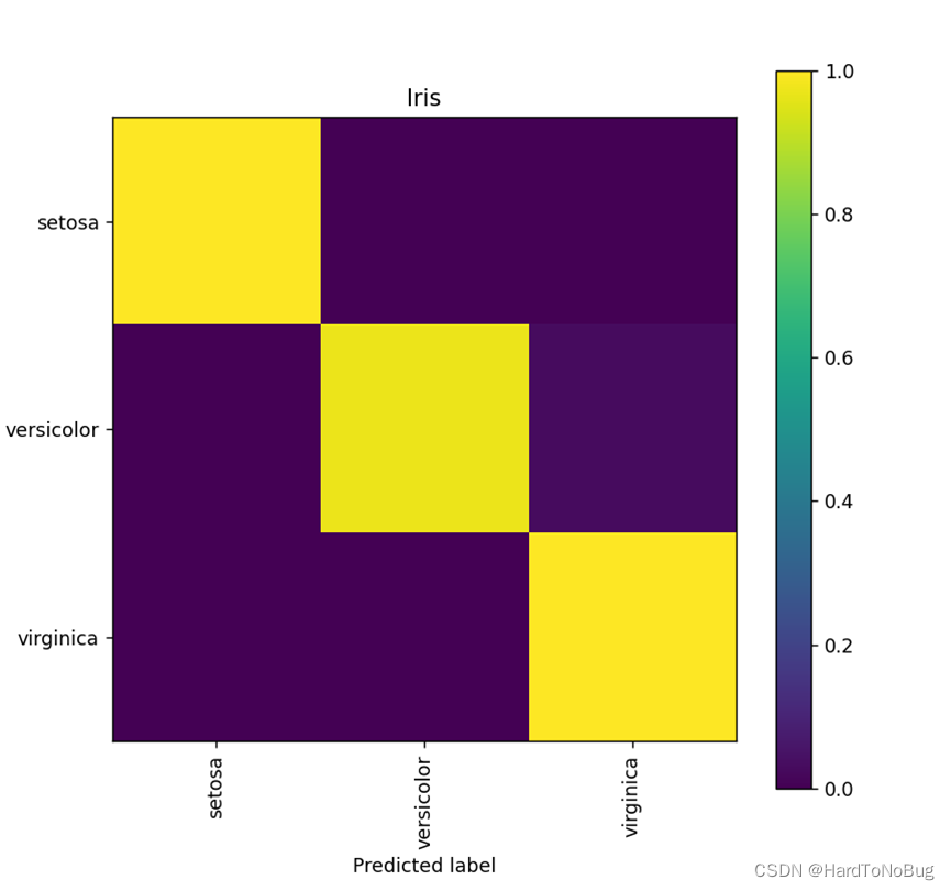
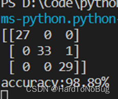
最终的结果应该是会在95%~99%之间波动

本文内容由网友自发贡献，版权归原作者所有，本站不承担相应法律责任。如您发现有涉嫌抄袭侵权的内容，请联系:hwhale#tublm.com(使用前将#替换为@)