今晚又实战了一个小案例,把它总结出来:有些人利用信用卡进行诈骗等活动,如何根据用户的行为,来判断该用户的信用卡账单涉嫌欺诈呢?数据集见及链接: 在这个数据集中,由于原始数据有一定的隐私,因此,每一列(即特征)的名称并没有给出。
一开始,还是导入库:
import numpy as np
import pandas as pd
import matplotlib.pyplot as plt

data = pd.read_csv('creditcard.csv')
#data.head(10)
print (data.shape)
我们发现,最后一列"Class"要么是 0 ,要么是 1,而且是 0 的样本很多,1 的样本很少。这也符合正常情况:利用信用卡欺诈的情况毕竟是少数,大多数人都是守法的公民。由于样本太多了,我们不可能去数 0 和 1 的个数到底是多少。因此,需要做一下统计:
count_class = pd.value_counts(data['Class'],sort = True).sort_index()
print (count_class)
输出结果为:
0 284315
1 492
Name: Class, dtype: int64
结果也显示了,0的个数远远多于1的个数。那么,这样就会使正负样本的个数严重失衡。为了解决这个问题,我们需要针对样本不均衡,提出两种解决方案:过采样和下采样。
在对样本处理之前,我们需要对样本中的数据先进行处理。我们发现,有一列为 Time ,这一列显然与咱们的训练结果没有直接或间接关系,因此需要把这一列去掉。我们还发现,在 v1 ~v28特征中,取值范围大致在 -1 ~ +1 之间,而Amount 这一类数值非常大,如果我们不对这一列进行处理,这一列对结果的影响,可能非常巨大。因此,要对这一列做标准化:使均值为0,方差为1。 此部分代码如下:
from sklearn.preprocessing import StandardScaler    #导入数据预处理模块
data['normAmount'] = StandardScaler().fit_transform(data['Amount'].values.reshape(-1,1))   # -1表示系统自动计算得到的行,1表示1列
data = data.drop(['Time','Amount'],axis = 1)  # 删除两列,axis =1表示按照列删除,即删除特征。而axis=0是按行删除,是删除样本
#print (data.head(3))
#print (data['normAmount'])
解决样本不均衡:两种方法可以采用——过采样和下采样。过采样是对少的样本(此例中是类别为 1 的样本)再多生成些,使 类别为 1 的样本和 0 的样本一样多。而下采样是指,随机选取类别为 0 的样本,是类别为 0 的样本和类别为 1 的样本一样少。下采样的代码如下:
X = data.ix[:,data.columns != 'Class'] #ix 是通过行号和行标签进行取值
y = data.ix[:,data.columns == 'Class']    # y 为标签,即类别
number_records_fraud = len(data[data.Class==1])  #统计异常值的个数
#print (number_records_fraud)  # 492 个
#print (data[data.Class == 1].index)
fraud_indices = np.array(data[data.Class == 1].index)   #统计欺诈样本的下标,并变成矩阵的格式
#print (fraud_indices)
normal_indices = data[data.Class == 0].index   # 记录正常值的索引
random_normal_indices =np.random.choice(normal_indices,number_records_fraud,replace = False) # 从正常值的索引中,选择和异常值相等个数的样本
random_normal_indices = np.array(random_normal_indices)
#print (len(random_normal_indices))  #492 个

under_sample_indices = np.concatenate([fraud_indices,random_normal_indices])  # 将正负样本的索引进行组合
#print (under_sample_indices)   # 984个
under_sample_data = data.iloc[under_sample_indices,:]  # 按照索引进行取值
X_undersample = under_sample_data.iloc[:,under_sample_data.columns != 'Class']  #下采样后的训练集
y_undersample = under_sample_data.iloc[:,under_sample_data.columns == 'Class']   #下采样后的标签

print (len(under_sample_data[under_sample_data.Class==1])/len(under_sample_data)) # 正负样本的比例都是 0.5
下一步:交叉验证。交叉验证可以辅助调参,使模型的评估效果更好。举个例子,对于一个数据集,我们需要拿出一部分作为训练集(比如 80%),计算我们需要的参数。需要拿出剩下的样本,作为测试集,评估我们的模型的好坏。但是,对于训练集,我们也并不是一股脑地拿去训练。比如把训练集又分成三部分:1,2,3.第 1 部分和第 2 部分作为训练集,第 3 部分作为验证集。然后,再把第 2 部分和第 3 部分作为训练集,第 1 部分作为验证集,然后,再把第 1部分和第 3 部分作为训练集,第 2 部分作为验证集。
from sklearn.cross_validation import train_test_split   # 导入交叉验证模块的数据切分
X_train,X_test,y_train,y_test = train_test_split(X,y,test_size = 0.3,random_state = 0) # 返回 4 个值
#print (len(X_train)+len(X_test))
#print (len(X))

X_undersample_train,X_undersample_test,y_undersample_train,y_undersample_train = train_test_split(X_undersample,y_undersample,test_size = 0.3,random_state = 0)
print (len(X_undersample_train)+len(X_undersample_test))
print (len(X_undersample))
我们需要注意,对数据进行切分,既要对原始数据进行一定比例的切分,测试时能用到;又要对下采样后的样本进行切分,训练的时候用。而且,切分之前,每次都要进行洗牌。
下一步:模型评估。利用交叉验证,选择较好的参数
#Recall = TP/(TP+FN)
from sklearn.linear_model import LogisticRegression  #
from sklearn.cross_validation import KFold, cross_val_score  #
from sklearn.metrics import confusion_matrix,recall_score,classification_report #
先说一个召回率 Recall,这个recall 是需要依据问题本身的含义的,比如,本例中让预测异常值,假设有100个样本,95个正常,5个异常。实际中,对于异常值,预测出来4个,所以,精度就是 80%。也就是说,我需要召回 5 个,实际召回 4 个。
引入四个小定义:TP、TN、FP、FN。
TP,即 True Positive ,判断成了正例,判断正确;把正例判断为正例了
TN,即 True negative, 判断成了负例,判断正确,这叫去伪;把负例判断为负例了
FP,即False Positive ,判断成了正例,但是判断错了,也就是把负例判断为正例了
FN ,即False negative ,判断成了负例,但是判断错了,也就是把正例判断为负例了
正则化惩罚项:为了提高模型的泛化能力,需要加了诸如 L1 、L2惩罚项一类的东西,对于这一部分内容,请参见我以前的博客。
def printing_Kfold_scores(x_train_data,y_train_data):
    fold = KFold(len(y_train_data),5,shuffle=False)
    c_param_range = [0.01,0.1,1,10,100] # 惩罚力度参数
    results_table = pd.DataFrame(index = range(len(c_param_range),2),columns = ['C_parameter','Mean recall score'])
    results_table['C_parameter'] = c_param_range

    # k折交叉验证有两个;列表: train_indices = indices[0], test_indices = indices[1]
    j = 0
    for c_param in c_param_range:  #
        print('------------------------------------------')
        print('C parameter:',c_param)
        print('-------------------------------------------')
        print('')

        recall_accs = []

        for iteration, indices in enumerate(fold,start=1):   #循环进行交叉验证

            # Call the logistic regression model with a certain C parameter
            lr = LogisticRegression(C = c_param, penalty = 'l1')  #实例化逻辑回归模型,L1 正则化

            # Use the training data to fit the model. In this case, we use the portion of the fold to train the model
            # with indices[0]. We then predict on the portion assigned as the 'test cross validation' with indices[1]
            lr.fit(x_train_data.iloc[indices[0],:],y_train_data.iloc[indices[0],:].values.ravel())#  套路:使训练模型fit模型

            # Predict values using the test indices in the training data
            y_pred_undersample = lr.predict(x_train_data.iloc[indices[1],:].values)# 利用交叉验证进行预测

            # Calculate the recall score and append it to a list for recall scores representing the current c_parameter
            recall_acc = recall_score(y_train_data.iloc[indices[1],:].values,y_pred_undersample) #评估预测结果
            recall_accs.append(recall_acc)
            print('Iteration ', iteration,': recall score = ', recall_acc)

        # The mean value of those recall scores is the metric we want to save and get hold of.
        results_table.ix[j,'Mean recall score'] = np.mean(recall_accs)
        j += 1
        print('')
        print('Mean recall score ', np.mean(recall_accs))
        print('')

    best_c = results_table.loc[results_table['Mean recall score'].idxmax()]['C_parameter']

    # Finally, we can check which C parameter is the best amongst the chosen.
    print('*********************************************************************************')
    print('Best model to choose from cross validation is with C parameter = ', best_c)
    print('*********************************************************************************')

    return best_c
运行:
best_c = printing_Kfold_scores(X_train_undersample,y_train_undersample)
上面程序中,我们选择进行 5 折的交叉验证,对应地选择了5个惩罚力度参数:0.01,0.1,1,10,100。不同的惩罚力度参数,得到的 Recall 是不一样的。
C parameter: 0.01
-------------------------------------------
Iteration 1 : recall score = 0.958904109589
Iteration 2 : recall score = 0.917808219178
Iteration 3 : recall score = 1.0
Iteration 4 : recall score = 0.972972972973
Iteration 5 : recall score = 0.954545454545
Mean recall score 0.960846151257
-------------------------------------------
C parameter: 0.1
-------------------------------------------
Iteration 1 : recall score = 0.835616438356
Iteration 2 : recall score = 0.86301369863
Iteration 3 : recall score = 0.915254237288
Iteration 4 : recall score = 0.932432432432
Iteration 5 : recall score = 0.878787878788
Mean recall score 0.885020937099
-------------------------------------------
C parameter: 1
-------------------------------------------
Iteration 1 : recall score = 0.835616438356
Iteration 2 : recall score = 0.86301369863
Iteration 3 : recall score = 0.966101694915
Iteration 4 : recall score = 0.945945945946
Iteration 5 : recall score = 0.893939393939
Mean recall score 0.900923434357
-------------------------------------------
C parameter: 10
-------------------------------------------
Iteration 1 : recall score = 0.849315068493
Iteration 2 : recall score = 0.86301369863
Iteration 3 : recall score = 0.966101694915
Iteration 4 : recall score = 0.959459459459
Iteration 5 : recall score = 0.893939393939
Mean recall score 0.906365863087
-------------------------------------------
C parameter: 100
-------------------------------------------
Iteration 1 : recall score = 0.86301369863
Iteration 2 : recall score = 0.86301369863
Iteration 3 : recall score = 0.966101694915
Iteration 4 : recall score = 0.959459459459
Iteration 5 : recall score = 0.893939393939
Mean recall score 0.909105589115
*********************************************************************************
Best model to choose from cross validation is with C parameter = 0.01
*********************************************************************************
接下来,介绍混淆矩阵。虽然上面的
def plot_confusion_matrix(cm, classes,
                          title='Confusion matrix',
                          cmap=plt.cm.Blues):
    """
    This function prints and plots the confusion matrix.
    """
    plt.imshow(cm, interpolation='nearest', cmap=cmap)
    plt.title(title)
    plt.colorbar()
    tick_marks = np.arange(len(classes))
    plt.xticks(tick_marks, classes, rotation=0)
    plt.yticks(tick_marks, classes)

    thresh = cm.max() / 2.
    for i, j in itertools.product(range(cm.shape[0]), range(cm.shape[1])):
        plt.text(j, i, cm[i, j],
                 horizontalalignment="center",
                 color="white" if cm[i, j] > thresh else "black")

    plt.tight_layout()
    plt.ylabel('True label')
    plt.xlabel('Predicted label')
混淆矩阵的计算:
import itertools
lr = LogisticRegression(C = best_c, penalty = 'l1')
lr.fit(X_train_undersample,y_train_undersample.values.ravel())
y_pred_undersample = lr.predict(X_test_undersample.values)

# Compute confusion matrix
cnf_matrix = confusion_matrix(y_test_undersample,y_pred_undersample)
np.set_printoptions(precision=2)

print("Recall metric in the testing dataset: ", cnf_matrix[1,1]/(cnf_matrix[1,0]+cnf_matrix[1,1]))

# Plot non-normalized confusion matrix
class_names = [0,1]
plt.figure()
plot_confusion_matrix(cnf_matrix
                      , classes=class_names
                      , title='Confusion matrix')
plt.show()
结果如下:
Recall metric in the testing dataset: 0.931972789116
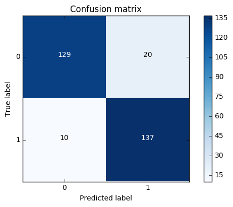
我们发现:
lr = LogisticRegression(C = best_c, penalty = 'l1')
lr.fit(X_train_undersample,y_train_undersample.values.ravel())
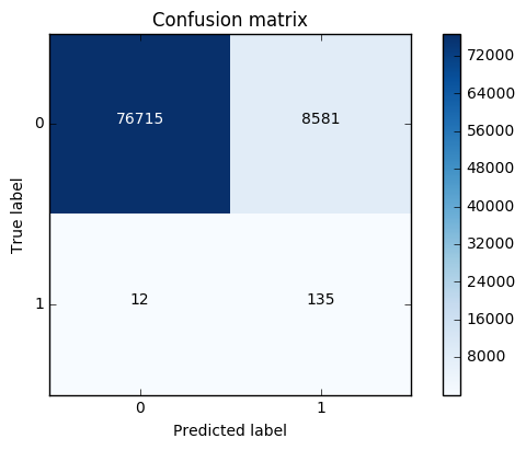
y_pred = lr.predict(X_test.values)
# Compute confusion matrix
cnf_matrix = confusion_matrix(y_test,y_pred)
np.set_printoptions(precision=2)
print("Recall metric in the testing dataset: ", cnf_matrix[1,1]/(cnf_matrix[1,0]+cnf_matrix[1,1]))
# Plot non-normalized confusion matrix
class_names = [0,1]
plt.figure()
plot_confusion_matrix(cnf_matrix
, classes=class_names
, title='Confusion matrix')
plt.show()
Recall metric in the testing dataset: 0.918367346939
运行:
best_c = printing_Kfold_scores(X_train,y_train)
C parameter: 0.01
-------------------------------------------
Iteration 1 : recall score = 0.492537313433
Iteration 2 : recall score = 0.602739726027
Iteration 3 : recall score = 0.683333333333
Iteration 4 : recall score = 0.569230769231
Iteration 5 : recall score = 0.45
Mean recall score 0.559568228405
-------------------------------------------
C parameter: 0.1
-------------------------------------------
Iteration 1 : recall score = 0.567164179104
Iteration 2 : recall score = 0.616438356164
Iteration 3 : recall score = 0.683333333333
Iteration 4 : recall score = 0.584615384615
Iteration 5 : recall score = 0.525
Mean recall score 0.595310250644
-------------------------------------------
C parameter: 1
-------------------------------------------
Iteration 1 : recall score = 0.55223880597
Iteration 2 : recall score = 0.616438356164
Iteration 3 : recall score = 0.716666666667
Iteration 4 : recall score = 0.615384615385
Iteration 5 : recall score = 0.5625
Mean recall score 0.612645688837
-------------------------------------------
C parameter: 10
-------------------------------------------
Iteration 1 : recall score = 0.55223880597
Iteration 2 : recall score = 0.616438356164
Iteration 3 : recall score = 0.733333333333
Iteration 4 : recall score = 0.615384615385
Iteration 5 : recall score = 0.575
Mean recall score 0.61847902217
-------------------------------------------
C parameter: 100
-------------------------------------------
Iteration 1 : recall score = 0.55223880597
Iteration 2 : recall score = 0.616438356164
Iteration 3 : recall score = 0.733333333333
Iteration 4 : recall score = 0.615384615385
Iteration 5 : recall score = 0.575
Mean recall score 0.61847902217
*********************************************************************************
Best model to choose from cross validation is with C parameter = 10.0
*********************************************************************************
我们发现:
lr = LogisticRegression(C = best_c, penalty = 'l1')
lr.fit(X_train,y_train.values.ravel())
y_pred_undersample = lr.predict(X_test.values)

# Compute confusion matrix
cnf_matrix = confusion_matrix(y_test,y_pred_undersample)
np.set_printoptions(precision=2)

print("Recall metric in the testing dataset: ", cnf_matrix[1,1]/(cnf_matrix[1,0]+cnf_matrix[1,1]))

# Plot non-normalized confusion matrix
class_names = [0,1]
plt.figure()
plot_confusion_matrix(cnf_matrix
                      , classes=class_names
                      , title='Confusion matrix')
plt.show()
结果:
Recall metric in the testing dataset: 0.619047619048

我们发现:
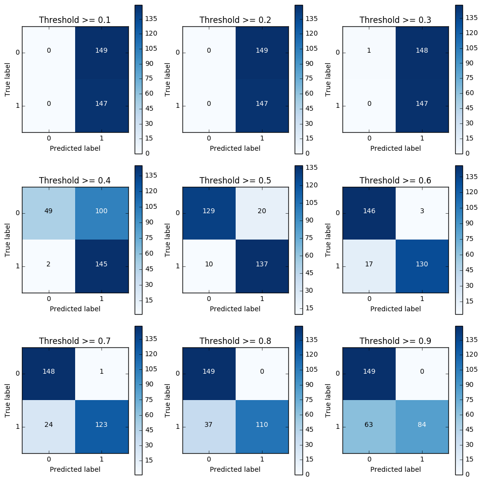
设置阈值。
lr = LogisticRegression(C = 0.01, penalty = 'l1')
lr.fit(X_train_undersample,y_train_undersample.values.ravel())
y_pred_undersample_proba = lr.predict_proba(X_test_undersample.values)#原来时预测类别值,而此处是预测概率。方便后续比较

thresholds = [0.1,0.2,0.3,0.4,0.5,0.6,0.7,0.8,0.9]

plt.figure(figsize=(10,10))

j = 1
for i in thresholds:
    y_test_predictions_high_recall = y_pred_undersample_proba[:,1] > i

    plt.subplot(3,3,j)
    j += 1

    # Compute confusion matrix
    cnf_matrix = confusion_matrix(y_test_undersample,y_test_predictions_high_recall)
    np.set_printoptions(precision=2)

    print("Recall metric in the testing dataset: ", cnf_matrix[1,1]/(cnf_matrix[1,0]+cnf_matrix[1,1]))

    # Plot non-normalized confusion matrix
    class_names = [0,1]
    plot_confusion_matrix(cnf_matrix
                          , classes=class_names
                          , title='Threshold >= %s'%i)
结果:
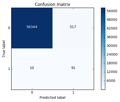
换种思路,采用上采样,进行数据增广。
import pandas as pd
from imblearn.over_sampling import SMOTE #上采样库,导入SMOTE算法
from sklearn.ensemble import RandomForestClassifier
from sklearn.metrics import confusion_matrix
from sklearn.model_selection import train_test_split
credit_cards=pd.read_csv('creditcard.csv')

columns=credit_cards.columns
# The labels are in the last column ('Class'). Simply remove it to obtain features columns
features_columns=columns.delete(len(columns)-1)

features=credit_cards[features_columns]
labels=credit_cards['Class']
features_train, features_test, labels_train, labels_test = train_test_split(features,
                                                                            labels,
                                                                            test_size=0.2,
                                                                            random_state=0)
oversampler=SMOTE(random_state=0)  #实例化参数,只对训练集增广,测试集不动
os_features,os_labels=oversampler.fit_sample(features_train,labels_train)# 使 0 和 1 样本相等
os_features = pd.DataFrame(os_features)
os_labels = pd.DataFrame(os_labels)
best_c = printing_Kfold_scores(os_features,os_labels)
参数选择的结果:
C parameter: 0.01
-------------------------------------------
Iteration 1 : recall score = 0.890322580645
Iteration 2 : recall score = 0.894736842105
Iteration 3 : recall score = 0.968861347792
Iteration 4 : recall score = 0.957595541926
Iteration 5 : recall score = 0.958430881173
Mean recall score 0.933989438728
-------------------------------------------
C parameter: 0.1
-------------------------------------------
Iteration 1 : recall score = 0.890322580645
Iteration 2 : recall score = 0.894736842105
Iteration 3 : recall score = 0.970410534469
Iteration 4 : recall score = 0.959980655302
Iteration 5 : recall score = 0.960178498807
Mean recall score 0.935125822266
-------------------------------------------
C parameter: 1
-------------------------------------------
Iteration 1 : recall score = 0.890322580645
Iteration 2 : recall score = 0.894736842105
Iteration 3 : recall score = 0.970454796946
Iteration 4 : recall score = 0.96014552489
Iteration 5 : recall score = 0.960596168431
Mean recall score 0.935251182603
-------------------------------------------
C parameter: 10
-------------------------------------------
Iteration 1 : recall score = 0.890322580645
Iteration 2 : recall score = 0.894736842105
Iteration 3 : recall score = 0.97065397809
Iteration 4 : recall score = 0.960343368396
Iteration 5 : recall score = 0.960530220596
Mean recall score 0.935317397966
-------------------------------------------
C parameter: 100
-------------------------------------------
Iteration 1 : recall score = 0.890322580645
Iteration 2 : recall score = 0.894736842105
Iteration 3 : recall score = 0.970543321899
Iteration 4 : recall score = 0.960211472725
Iteration 5 : recall score = 0.960903924995
Mean recall score 0.935343628474
*********************************************************************************
Best model to choose from cross validation is with C parameter = 100.0
*********************************************************************************
打印一下混淆矩阵的结果:
lr = LogisticRegression(C = best_c, penalty = 'l1')
lr.fit(os_features,os_labels.values.ravel())
y_pred = lr.predict(features_test.values)

# Compute confusion matrix
cnf_matrix = confusion_matrix(labels_test,y_pred)
np.set_printoptions(precision=2)

print("Recall metric in the testing dataset: ", cnf_matrix[1,1]/(cnf_matrix[1,0]+cnf_matrix[1,1]))

# Plot non-normalized confusion matrix
class_names = [0,1]
plt.figure()
plot_confusion_matrix(cnf_matrix
                      , classes=class_names
                      , title='Confusion matrix')
plt.show()
Recall metric in the testing dataset: 0.90099009901
总结:
本文内容由网友自发贡献,版权归原作者所有,本站不承担相应法律责任。如您发现有涉嫌抄袭侵权的内容,请联系:hwhale#tublm.com(使用前将#替换为@)