Regylaerization Term 正则化方式有 L1 和 L2 正则项两种。其中 L2 正则项又被称为权值衰减(weight decay)。
其中Cost可以用Loss表示,然后λ是超参数,1/2是为了消除求导带的一个系数。
通常,λ取值范围为(0,1),所以wi(1−λ)变小了。也就是为什么叫权重衰减的原因,变小了嘛。
当没有正则项时:
O
b
j
=
L
o
s
s
,
w
i
+
1
=
w
i
−
∂
o
b
j
∂
w
i
=
w
i
−
∂
L
o
s
s
∂
w
i
\boldsymbol{O} \boldsymbol{b} \boldsymbol{j}=\boldsymbol{L} \boldsymbol{o} \boldsymbol{s} \boldsymbol{s},w_{i+1}=w_{i}-\frac{\partial o b j}{\partial w_{i}}=w_{i}-\frac{\partial L o s s}{\partial w_{i}}
Obj=Loss,wi+1=wi−∂wi∂obj=wi−∂wi∂Loss。
当使用 L2 正则项时,
O
b
j
=
L
o
s
s
+
λ
2
∗
∑
i
N
w
i
2
,
w
i
+
1
=
w
i
−
∂
o
b
j
∂
w
i
=
w
i
−
(
∂
L
o
s
s
∂
w
i
+
λ
∗
w
i
)
=
w
i
(
1
−
λ
)
−
∂
L
o
s
s
∂
w
i
\boldsymbol{O} \boldsymbol{b} \boldsymbol{j}=\boldsymbol{L} \boldsymbol{o} \boldsymbol{s} \boldsymbol{s}+\frac{\lambda}{2} * \sum_{i}^{N} \boldsymbol{w}_{i}^{2},\begin{aligned} w_{i+1}=w_{i}-\frac{\partial o b j}{\partial w_{i}} &=w_{i}-\left(\frac{\partial L o s s}{\partial w_{i}}+\lambda * w_{i}\right) =w_{i}(1-\lambda)-\frac{\partial L o s s}{\partial w_{i}} \end{aligned}
Obj=Loss+2λ∗∑iNwi2,wi+1=wi−∂wi∂obj=wi−(∂wi∂Loss+λ∗wi)=wi(1−λ)−∂wi∂Loss,其中
0
<
λ
<
1
0 < \lambda < 1
0<λ<1,所以具有权值衰减的作用。
defstep(self, closure=None):"""Performs a single optimization step.
Arguments:
closure (callable, optional): A closure that reevaluates the model
and returns the loss.
"""
loss =Noneif closure isnotNone:
loss = closure()for group in self.param_groups:
weight_decay = group['weight_decay']
momentum = group['momentum']
dampening = group['dampening']
nesterov = group['nesterov']for p in group['params']:if p.grad isNone:continue
d_p = p.grad.data
if weight_decay !=0:
d_p.add_(weight_decay, p.data).........
p.data.add_(-group['lr'], d_p)
可以看到:dp 是计算得到的梯度,如果 weight decay 不为 0,那么更新
d
p
=
d
p
+
w
e
i
g
h
t
d
e
c
a
y
×
p
.
d
a
t
a
d_p=dp+weight_{decay} \times p.data
dp=dp+weightdecay×p.data,对应公式:
(
∂
L
o
s
s
∂
w
i
+
λ
∗
w
i
)
\left(\frac{\partial L o s s}{\partial w{i}}+\lambda * w_{i}\right)
(∂wi∂Loss+λ∗wi)。最后一行是根据梯度更新权值。
假设输入的 mini-batch 数据是
B
=
{
x
1
…
m
}
\mathcal{B}=\left\{x_{1 \dots m}\right\}
B={x1…m},Batch Normalization 的可学习参数是
γ
\gamma
γ,
β
\beta
β,步骤如下:
求 mini-batch 的均值:
μ
B
←
1
m
∑
i
=
1
m
x
i
\mu_{\mathcal{B}} \leftarrow \frac{1}{m} \sum_{i=1}^{m} x_{i}
μB←m1∑i=1mxi
求 mini-batch 的方差:
σ
B
2
←
1
m
∑
i
=
1
(
x
i
−
μ
B
)
2
\sigma_{\mathcal{B}}^{2} \leftarrow \frac{1}{m} \sum_{i=1}\left(x_{i}-\mu_{\mathcal{B}}\right)^{2}
σB2←m1∑i=1(xi−μB)2
标准化:
x
^
i
←
x
i
−
μ
B
σ
B
2
+
ϵ
\widehat{x}_{i} \leftarrow \frac{x_{i}-\mu_{\mathcal{B}}}{\sqrt{\sigma_{B}^{2}+\epsilon}}
xi←σB2+ϵxi−μB,其中
ϵ
\epsilon
ϵ 是放置分母为 0 的一个数
affine transform(缩放和平移):
y
i
←
γ
x
^
i
+
β
≡
B
N
γ
,
β
(
x
i
)
y_{i} \leftarrow \gamma \widehat{x}_{i}+\beta \equiv \mathrm{B} \mathrm{N}_{\gamma, \beta}\left(x_{i}\right)
yi←γxi+β≡BNγ,β(xi),这个操作可以增强模型的 capacity,也就是让模型自己判断是否要对数据进行标准化,进行多大程度的标准化。如果
γ
=
σ
B
2
,
β
=
μ
B
\gamma= \sqrt{\sigma_{B}^{2}},\beta=\mu_{\mathcal{B}}
γ=σB2,β=μB,那么就实现了恒等映射。
参考: Batch Normalization: Accelerating Deep Network Training by Reducing Internal Covariate Shift 在训练过程中,数据需要经过多层的网络,如果数据在前向传播的过程中,尺度发生了变化,可能会导致梯度爆炸或者梯度消失,从而导致模型难以收敛。
Batch Normalization 层一般在激活函数前一层。
下面的代码打印一个网络的每个网络层的输出,在没有进行初始化时,数据尺度越来越小。
import torch
import numpy as np
import torch.nn as nn
from common_tools import set_seed
set_seed(1)# 设置随机种子classMLP(nn.Module):def__init__(self, neural_num, layers=100):super(MLP, self).__init__()
self.linears = nn.ModuleList([nn.Linear(neural_num, neural_num, bias=False)for i inrange(layers)])
self.bns = nn.ModuleList([nn.BatchNorm1d(neural_num)for i inrange(layers)])
self.neural_num = neural_num
defforward(self, x):for(i, linear), bn inzip(enumerate(self.linears), self.bns):
x = linear(x)# x = bn(x)
x = torch.relu(x)if torch.isnan(x.std()):print("output is nan in {} layers".format(i))breakprint("layers:{}, std:{}".format(i, x.std().item()))return x
definitialize(self):for m in self.modules():ifisinstance(m, nn.Linear):# method 1# nn.init.normal_(m.weight.data, std=1) # normal: mean=0, std=1# method 2 kaiming
nn.init.kaiming_normal_(m.weight.data)
neural_nums =256
layer_nums =100
batch_size =16
net = MLP(neural_nums, layer_nums)# net.initialize()
inputs = torch.randn((batch_size, neural_nums))# normal: mean=0, std=1
output = net(inputs)print(output)
classLeNet_bn(nn.Module):def__init__(self, classes):super(LeNet_bn, self).__init__()
self.conv1 = nn.Conv2d(3,6,5)
self.bn1 = nn.BatchNorm2d(num_features=6)
self.conv2 = nn.Conv2d(6,16,5)
self.bn2 = nn.BatchNorm2d(num_features=16)
self.fc1 = nn.Linear(16*5*5,120)
self.bn3 = nn.BatchNorm1d(num_features=120)
self.fc2 = nn.Linear(120,84)
self.fc3 = nn.Linear(84, classes)defforward(self, x):
out = self.conv1(x)
out = self.bn1(out)
out = F.relu(out)
out = F.max_pool2d(out,2)
out = self.conv2(out)
out = self.bn2(out)
out = F.relu(out)
out = F.max_pool2d(out,2)
out = out.view(out.size(0),-1)
out = self.fc1(out)
out = self.bn3(out)
out = F.relu(out)
out = F.relu(self.fc2(out))
out = self.fc3(out)return out
带 bn 层的网络,并且不使用 kaiming 初始化权值,训练过程如下:
虽然训练过程中,训练集的 loss 也有激增,但只是增加到 0.4,非常稳定。
2.2.Batch Normalization in PyTorch
在 PyTorch 中,有 3 个 Batch Normalization 类
nn.BatchNorm1d(),输入数据的形状是
B
×
C
×
1
D
_
f
e
a
t
u
r
e
B \times C \times 1D\_feature
B×C×1D_feature
nn.BatchNorm2d(),输入数据的形状是
B
×
C
×
2
D
_
f
e
a
t
u
r
e
B \times C \times 2D\_feature
B×C×2D_feature
nn.BatchNorm3d(),输入数据的形状是
B
×
C
×
3
D
_
f
e
a
t
u
r
e
B \times C \times 3D\_feature
B×C×3D_feature
输入数据的形状是
B
×
C
×
1
D
_
f
e
a
t
u
r
e
B \times C \times 1D\_feature
B×C×1D_feature。在下面的例子中,数据的维度是:(3, 5, 1),表示一个 mini-batch 有 3 个样本,每个样本有 5 个特征,每个特征的维度是 1。那么就会计算 5 个均值和方差,分别对应每个特征维度。momentum 设置为 0.3,第一次的均值和方差默认为 0 和 1。输入两次 mini-batch 的数据。
第一次 bn 层的均值计算:
r
u
n
n
i
n
g
_
m
e
a
n
=
(
1
−
m
o
m
e
n
t
u
m
)
×
p
r
e
_
r
u
n
n
i
n
g
_
m
e
a
n
+
m
o
m
e
n
t
u
m
×
m
e
a
n
_
t
=
(
1
−
0.3
)
×
0
+
0.3
×
2
=
0.6
running\_{mean}=(1-momentum) \times pre\_running\_mean + momentum \times mean\_t =(1-0.3) \times 0 + 0.3 \times 2 =0.6
running_mean=(1−momentum)×pre_running_mean+momentum×mean_t=(1−0.3)×0+0.3×2=0.6
第二次 bn 层的均值计算:
r
u
n
n
i
n
g
_
m
e
a
n
=
(
1
−
m
o
m
e
n
t
u
m
)
×
p
r
e
_
r
u
n
n
i
n
g
_
m
e
a
n
+
m
o
m
e
n
t
u
m
×
m
e
a
n
_
t
=
(
1
−
0.3
)
×
0.6
+
0.3
×
2
=
1.02
running\_mean=(1-momentum) \times pre\_running\_mean + momentum \times mean\_t =(1-0.3) \times 0.6 + 0.3 \times 2 =1.02
running_mean=(1−momentum)×pre_running_mean+momentum×mean_t=(1−0.3)×0.6+0.3×2=1.02
输入数据的形状是
B
×
C
×
2
D
_
f
e
a
t
u
r
e
B \times C \times 2D\_feature
B×C×2D_feature。在下面的例子中,数据的维度是:(3, 3, 2, 2),表示一个 mini-batch 有 3 个样本,每个样本有 3 个特征,每个特征的维度是
1
×
2
1 \times 2
1×2。那么就会计算 3 个均值和方差,分别对应每个特征维度。momentum 设置为 0.3,第一次的均值和方差默认为 0 和 1。输入两次 mini-batch 的数据。
数据如下图:
如上图所示,样本数为3,即B=3,特征数为3,每个特征是2×2,因此输入为3×3×2×2
代码如下:
batch_size =3
num_features =3
momentum =0.3
features_shape =(2,2)
feature_map = torch.ones(features_shape)# 2D
feature_maps = torch.stack([feature_map*(i+1)for i inrange(num_features)], dim=0)# 3D
feature_maps_bs = torch.stack([feature_maps for i inrange(batch_size)], dim=0)# 4D# print("input data:\n{} shape is {}".format(feature_maps_bs, feature_maps_bs.shape))
bn = nn.BatchNorm2d(num_features=num_features, momentum=momentum)
running_mean, running_var =0,1for i inrange(2):
outputs = bn(feature_maps_bs)print("\niter:{}, running_mean: {}".format(i, bn.running_mean))print("iter:{}, running_var: {}".format(i, bn.running_var))print("iter:{}, weight: {}".format(i, bn.weight.data.numpy()))print("iter:{}, bias: {}".format(i, bn.bias.data.numpy()))
输入数据的形状是
B
×
C
×
3
D
_
f
e
a
t
u
r
e
B \times C \times 3D\_feature
B×C×3D_feature。在下面的例子中,数据的维度是:(3, 2, 2, 2, 3),表示一个 mini-batch 有 3 个样本,每个样本有 2 个特征,每个特征的维度是
2
×
2
×
3
2 \times 2 \times 3
2×2×3。那么就会计算 2 个均值和方差,分别对应每个特征维度。momentum 设置为 0.3,第一次的均值和方差默认为 0 和 1。输入两次 mini-batch 的数据。
数据如下图:
nn.BatchNorm3d input= Bx特征数x3d特征(B为 batch 的样本数目)
如上图所示,样本数为3,即B=3,特征数为3,每个特征是2×2×3,因此输入为3×3×2×2×3
代码如下:
batch_size =3
num_features =3
momentum =0.3
features_shape =(2,2,3)
feature = torch.ones(features_shape)# 3D
feature_map = torch.stack([feature *(i +1)for i inrange(num_features)], dim=0)# 4D
feature_maps = torch.stack([feature_map for i inrange(batch_size)], dim=0)# 5D# print("input data:\n{} shape is {}".format(feature_maps, feature_maps.shape))
bn = nn.BatchNorm3d(num_features=num_features, momentum=momentum)
running_mean, running_var =0,1for i inrange(2):
outputs = bn(feature_maps)print("\niter:{}, running_mean.shape: {}".format(i, bn.running_mean.shape))print("iter:{}, running_var.shape: {}".format(i, bn.running_var.shape))print("iter:{}, weight.shape: {}".format(i, bn.weight.shape))print("iter:{}, bias.shape: {}".format(i, bn.bias.shape))
normalized_shape:该层特征的形状,可以取
C
×
H
×
W
、
H
×
W
、
W
C \times H \times W、H \times W、W
C×H×W、H×W、W
eps:标准化时的分母修正项
elementwise_affine:是否需要逐个样本 affine transform
下面代码中,输入数据的形状是
B
×
C
×
f
e
a
t
u
r
e
B \times C \times feature
B×C×feature,(8, 2, 3, 4),表示一个 mini-batch 有 8 个样本,每个样本有 2 个特征,每个特征的维度是
3
×
4
3 \times 4
3×4。那么就会计算 8 个均值和方差,分别对应每个样本。
batch_size =8
num_features =2
features_shape =(3,4)
feature_map = torch.ones(features_shape)# 2D
feature_maps = torch.stack([feature_map *(i +1)for i inrange(num_features)], dim=0)# 3D
feature_maps_bs = torch.stack([feature_maps for i inrange(batch_size)], dim=0)# 4D# feature_maps_bs shape is [8, 6, 3, 4], B * C * H * W# ln = nn.LayerNorm(feature_maps_bs.size()[1:], elementwise_affine=True)# ln = nn.LayerNorm(feature_maps_bs.size()[1:], elementwise_affine=False)# ln = nn.LayerNorm([6, 3, 4])
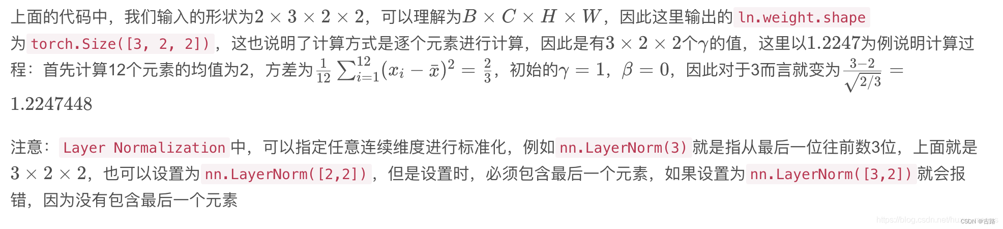
ln = nn.LayerNorm([2,3,4])
output = ln(feature_maps_bs)print("Layer Normalization")print(ln.weight.shape)print(feature_maps_bs[0,...])print(output[0,...])
下面代码中,输入数据的形状是
B
×
C
×
2
D
_
f
e
a
t
u
r
e
B \times C \times 2D\_feature
B×C×2D_feature,(3, 3, 2, 2),表示一个 mini-batch 有 3 个样本,每个样本有 3 个特征,每个特征的维度是
2
×
2
2 \times 2
2×2 。那么就会计算
3
×
3
3 \times 3
3×3 个均值和方差,分别对应每个样本的每个特征。如下图所示:
下面是代码:
batch_size =3
num_features =3
momentum =0.3
features_shape =(2,2)
feature_map = torch.ones(features_shape)# 2D
feature_maps = torch.stack([feature_map *(i +1)for i inrange(num_features)], dim=0)# 3D
feature_maps_bs = torch.stack([feature_maps for i inrange(batch_size)], dim=0)# 4Dprint("Instance Normalization")print("input data:\n{} shape is {}".format(feature_maps_bs, feature_maps_bs.shape))
instance_n = nn.InstanceNorm2d(num_features=num_features, momentum=momentum)for i inrange(1):
outputs = instance_n(feature_maps_bs)print(outputs)
下面代码中,输入数据的形状是
B
×
C
×
2
D
_
f
e
a
t
u
r
e
B \times C \times 2D\_feature
B×C×2D_feature,(2, 4, 3, 3),表示一个 mini-batch 有 2 个样本,每个样本有 4 个特征,每个特征的维度是
3
×
3
3 \times 3
3×3 。num_groups 设置为 2,那么就会计算
2
×
(
4
÷
2
)
2 \times (4 \div 2)
2×(4÷2) 个均值和方差,分别对应每个样本的每个特征。
batch_size =2
num_features =4
num_groups =2
features_shape =(2,2)
feature_map = torch.ones(features_shape)# 2D
feature_maps = torch.stack([feature_map *(i +1)for i inrange(num_features)], dim=0)# 3D
feature_maps_bs = torch.stack([feature_maps *(i +1)for i inrange(batch_size)], dim=0)# 4D
gn = nn.GroupNorm(num_groups, num_features)
outputs = gn(feature_maps_bs)print("Group Normalization")print(gn.weight.shape)print(outputs[0])