We begin at the beginning, with the law of averages, a greatly misunderstood and misquoted principle. In trading, the law of averages is most often referred to when an abnormally long series of losses is expected to be offset by an equal and opposite run of profits. It is equally wrong to expect a market that is currently overvalued or overbought to next become undervalued or oversold期望 当前 被高估或超买的 市场接下来会 被低估或超卖同样是错误的. That is not what is meant by the law of averages. Over a large sample, the bulk of events will be scattered分散 close to the average in such a way that the typical values overwhelm the abnormal events and cause them to be insignificant. 
Detecting outliers using visualizations(downsampled):  Figure 8.4 – Histogram showing extreme daily mean passenger rides极端的每日平均乘客乘车次数ts8_Outlier Detection_plotly_sns_text annot_modified z-score_hist_Tukey box_cdf_resample freq_Quanti_LIQING LIN的博客-CSDN博客
ts14_cb Local Outlier Factor Outlier_PyOD knn BallTree_justify_percentile_plotly text_IsolationForest_COPOD_MAD_PyCaret : ts14_cbLOFOutlier_PyOD knn BallTree_justify_percentile_plotly text_IsolationForest_COPOD_MAD_PyCaret_LIQING LIN的博客-CSDN博客
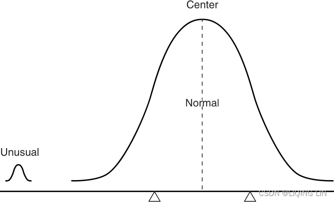
FIGURE 2.1 The Law of Averages. The normal cases overwhelm the unusual ones. It is not necessary for the extreme cases to alternate—one higher, the next lower—to create a balance.
This principle is illustrated in Figure 2.1, where the number of average items is extremely large, and the addition of a small abnormal grouping to one side of an average group of near-normal data does not affect the balance. It is the same as being the only passenger on a jumbo jet. Your weight is insignificant to the operation of the airplane and not noticed when you move about the cabin. A long run of profits, losses, or an unusually sustained price movement is simply a rare, abnormal event that will be offset over time by the overwhelming large number of normal events. Further discussion of this and how it affects trading can be found in “Gambling Techniques—The Theory of Runs,” Chapter 22.
Proper test procedures call for separating data into in-sample and out-of-sample sets. This will be discussed in Chapter 21, System Testing. For now, consider the most important points. All testing is overfitting the data, yet there is no way to find out if an idea or system works without testing it. By setting aside data that you have not seen to use for validation, you have a better chance that your idea will work before putting money on it.
There are many ways to select in-sample data. For example, if you have 20 years of price history, you might choose to use the first 10 years for testing and reserve the second 10 years for validation. But then markets change over time; they become more volatile and may be more or less trending. It might be best to use alternating periods of in-sample and out-of-sample data, in 2-year intervals最好每隔 2 年交替使用样本内和样本外数据, provided that you never look at the data during the out-of-sample periods. Alternating these periods may create a problem for continuous, long-term trends, but that will be resolved in Chapter 21.
The most important factor when reserving out-of-sample data is that you get only one chance to use it. Once you have done your best to create the rules for a trading program, you then run that program through the unseen data. If the results are successful then you can trade the system, but if it fails, then you are also done. You cannot look at the reasons why it failed and change the trading method to perform better. You would have introduced feedback, and your out-of-sample data is considered contaminated. The second try will always be better, but it is now overfitted.
Statisticians will say, “More is better.” The more data you test, the more reliable your results. Technical analysis is fortunate to be based on a perfect set of data. Each price that is recorded by the exchange, whether it’s IBM at the close of trading in New York on May 5, or the price of Eurodollar interest rates at 10:05 in Chicago, is a confirmed, precise value.
Remember that, when you use in-sample and out-of-sample data for development, you need more data. You will only get half the combinations and patterns when 50% of the data has been withheld当 50% 的数据被保留时,您将只能获得一半的组合和模式.
Most other statistical data are not as timely, not as precise, and not as reliable as the price and volume of stocks, futures, ETFs, and other exchange-traded products. Economic data, such as the Producer Price Index or Housing Starts, are released as monthly averages, and can be seasonally adjusted. A monthly average represents a broad range of numbers. In the case of the PPI, some producers may have paid less than the average of the prior month and some more, but the average was +0.02. The lack of a range of values, or a standard deviation of the component values, reduces the usefulness of the information. This statistical data is often revised in the following month; sometimes those revisions can be quite large. When working with the Department of Energy (DOE) weekly data releases, you will need to know the history of the exact numbers released as well as the revisions, if you are going to design a trading method that reacts to those reports. You may find that it is much easier to find the revised data, which is not what you really need.
If you use economic data, you must be aware of when that data is released. The United States is very precise and prompt but other countries can be months or years late in releasing data. If the input to your program is monthly data and comes from the CRB(Commodity Research Bureau Index) Yearbook, be sure that you check when that data was actually available.
When an average is used, it is necessary to have enough data to make that average accurate. Because much statistical data is gathered by sampling, particular care is given to accumulating a sufficient amount of representative data. This holds true with prices as well. Averaging a few prices, or analyzing small market moves, will show more erratic results. It is difficult to draw an accurate picture from a very small sample.
When using small, incomplete, or representative sets of data, the approximate error, or accuracy, of the sample can be found using the standard deviation. A large standard deviation indicates an extremely scattered set of points, which in turn makes the average less representative of the data. This process is called the testing of significance显着性检验. Accuracy increases as the number of items becomes larger, and the measurement of sample error becomes proportionately smaller![]()
Therefore, using only one item has a sample error样本误差 of 100%; with 4 items, the error is 50%. The size of the error is important to the reliability of any trading system. If a system has had only 4 trades, whether profits or losses, it is very difficult to draw any reliable conclusions about future performance. There must be sufficient trades to assure a comfortably small error factor. To reduce the error to 5%, there must be 400 trades. This presents a dilemma/dɪˈlemə/窘境 for a very slow trend-following method that may only generate two or three trades each year. To compensate for this, the identical method can be applied across many markets and the number of trades used collectively (more about this in Chapter 21).
The amount of data is a good estimate of its usefulness; however, the data should represent at least one bull market, one bear market, and some sideways periods. More than one of each is even better. If you were to use 10 years of daily S&P Index values from 1990 to 2000, or 25 years of 10-year Treasury notes through 2010, you would only see a bull market. A trading strategy would be profitable whenever it was a buyer, if you held the position long enough. Unless you included a variety of other price patterns, you would not be able to create a strategy that would survive a downturn in the market. Your results would be unrealistic.
The average can be misleading in other ways. Consider coffee, which rose from $0.40 to $2.00 per pound in one year. The average price of this product may appear to be $1.20; however, this would not account for the time that coffee was sold at various price levels. Table 2.1 divides the coffee price into four equal intervals, then shows that the time spent at these levels was uniformly opposite to the price rise. That is, prices remained at lower levels longer and at higher levels for shorter time periods, which is very normal price behavior.

When the time spent at each price level is included, it can be seen that the average price should be lower than $1.20. One way to calculate this, knowing the specific number of days in each interval, is by using a weighted average of the price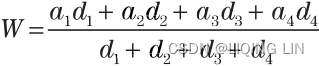 and its respective interval
This result can vary based on the number of time intervals used; however, it gives a better idea of the correct average price. There are two other averages for which time is an important element—the geometric mean and the harmonic mean.
The geometric mean represents a growth function in which a price change from 50 to 100 is as important as a change from 100 to 200. If there are n prices, ,
,
, . . . ,
, then the geometric mean is the nth root of the product of the prices
![]() or
or![]()
To solve this mathematically, rather than using a spreadsheet, the equation above can be changed to either of two forms: 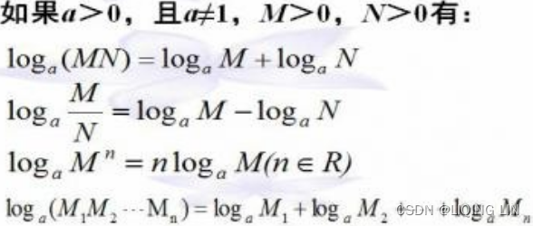
![]() or
or
The two solutions are equivalent. The term ln is the natural log, or log base e. (Note that there is some software where the function log actually is ln.) Using the price levels in Table 2.1
Disregarding the time intervals, and substituting into the first equation: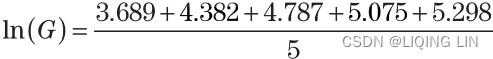
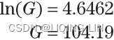 <==
<==
While the arithmetic mean, which is time-weighted, gave the value of 105.71, the geometric mean shows the average as 104.19.
The geometric mean has advantages in application to economics and prices.
and shows the relative distribution of prices as a function of comparable growth. Due to this property, the geometric mean is the best choice when averaging ratios that can be either fractions or percentages.
The quadratic mean is most often used for estimation of error. It is calculated as: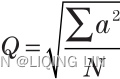
The quadratic mean is the square root of the mean of the square of the items (root-mean-square). It is most well known as the basis for the standard deviation().
 This will be discussed later in this chapter in the section “Moments of the Distribution: Variance, Skewness, and Kurtosis.”
The harmonic mean is another time-weighted average, but not biased toward higher or lower values as in the geometric mean. A simple example is to consider the average speed of a car that travels 4 miles at 20 mph, then 4 miles at 30 mph. An arithmetic mean would give 25 mph, without considering that 12 minutes
were spent at 20 mph and 8 minutes
at 30 mph.
The weighted average would give 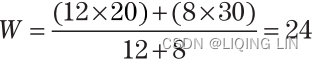
The harmonic mean is 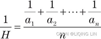
which can also be expressed as

For two or three values, the simpler form can be used: 
This allows the solution pattern to be seen. For the 20 and 30 mph rates of speed, the solution is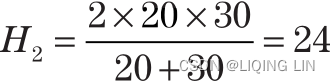
which is the same answer as the weighted average. Considering the original set of numbers again, the basic form of harmonic mean can be applied: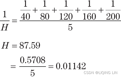
We might apply the harmonic mean to price swings, where the first swing moved 20 points over 12 days and the second swing moved 30 points over 8 days.
The measurement of distribution is very important because it tells you generally what to expect. We cannot know what tomorrow’s S&P trading range will be, but if the current price is 1200, then
The following measurements of distribution allow you to put a probability, or confidence level, on the chance of an event occurring.
In all of the statistics that follow, we will use a limited number of prices or—in some cases—individual trading profits and losses as the sample data. We want to measure the characteristics of our sample, finding the shape of the distribution, deciding how results of a smaller sample compare to a larger one, or how similar two samples are to each other. All of these measures will show that the smaller samples are less reliable, yet they can be still be used if you understand the size of the error or the difference in the shape of the distribution compared to the expected distribution of a larger sample.
import pandas as pd

wheat = pd.read_excel('TSM Monthly_W-PPI-DX (C2).xlsx',
                      index_col='Date'
                     )[['Wheat']]
wheat 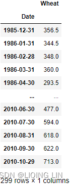
Log returns(log_return):![]() between two times 0 < s < t are normally distributed.
between two times 0 < s < t are normally distributed.
when s=t-1
import numpy as np
# Calculates the log returns
wheat['log_rtn'] = np.log( wheat['Wheat']/wheat['Wheat'].shift(1) )
wheat['Wheat(X)']=100

# estimated future price = (log return * 100) + previous price
for i in range(1,len(wheat)):
        wheat.iloc[i,
                   list(wheat.columns).index( 'Wheat(X)' )
                  ]= wheat['Wheat(X)'].iloc[i-1] + 100*wheat['log_rtn'].iloc[i]
#wheat['Wheat(X)'][0]=100
wheat
# plot the estimated future price
import matplotlib.pyplot as plt
import numpy as np
import matplotlib.dates as mdates

import datetime as dt
import matplotlib.ticker as ticker

fig, ax = plt.subplots(1, figsize=(8,6),#gridspec_kw={'height_ratios': [2, 1]}
                      )
ax.plot(wheat.index, wheat['Wheat(X)'].values,
        c='gray', lw=4
       )

ax.set_ylabel('Wheat Price(cents/bushhel)', fontsize=14)

# Enabling grid lines:
ax.grid(axis='y')
# ax.xaxis.set_major_formatter(mdates.DateFormatter('%m/%d/%Y'))
# ax.xaxis.set_major_locator( mdates.YearLocator() )
# ax.set_xticklabels( (pd.date_range( ax.get_xticklabels()[0].get_text(),
#                                    ax.get_xticklabels()[-1].get_text(),
#                                    freq="A"
#                                  )- pd.offsets.MonthBegin()
#                     ).date,
#                     rotation=90
#                   )

dates = [ dt.date(list(set(wheat.index.year))[0] + i, 12, 1)
              for i in range(len( set(wheat.index.year ) ))
        ]# datetime.date(1985, 12, 1), ... datetime.date(2010, 12, 1)]

tick_values = mdates.date2num(dates)#########
# [ 5813.  6178.  6543.  6909.  7274.  7639.  8004.  8370.  8735.  9100.
#   9465.  9831. 10196. 10561. 10926. 11292. 11657. 12022. 12387. 12753.
#  13118. 13483. 13848. 14214. 14579. 14944.]
ax.xaxis.set_major_locator( ticker.FixedLocator(tick_values) )

ax.set_xlim( xmin=dt.date( list(set(wheat.index.year))[0] ,
                           12,
                           1
                         )
           )
ax.xaxis.set_major_formatter(mdates.DateFormatter('%m/%d/%Y'))
# 12/01/1985, ... 12/01/2009
ax.set_xticklabels( [ label.get_text().replace('/0', '/')
                      for label in ax.get_xticklabels()
                    ],#remove the leading zero from a day in a Matplotlib tick label formatting
                    rotation=90
                  )
# ax.set_xticklabels( ax.get_xticklabels(),#remove the leading zero from a day in a Matplotlib tick label formatting
#                     rotation=90
#                   )
ax.set_yticks(np.arange(0, 300, 50), )
#ax.autoscale(enable=True, axis='x', tight=True)
ax.spines['right'].set_visible(False)
ax.spines['top'].set_visible(False)
plt.show() 
FIGURE 2.2 Wheat prices, 1985–2010.
VS
The frequency distribution (also called a histogram) is simple yet can give a good picture of the characteristics of the data. Theoretically, we expect commodity prices to spend more time at low price levels and only brief periods at high prices. That pattern is shown in Figure 2.2 for wheat during the past 25 years. The most frequent occurrences are at the price where the supply and demand are balanced, called equilibrium(equilibrium price : the price that balances quantity supplied and quantity demanded).
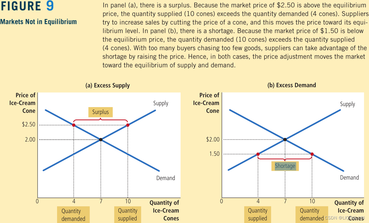
 When there is a shortage of supply(excess demand供不应求), or an unexpected demand需求意外, prices rise for a short time until either the demand is satisfied (which could happen if prices are too high), or supply increases to meet demand
(With too many buyers chasing too few goods, sellers can respond to the shortage by raising their prices without losing sales. These price increases cause the quantity demanded to fall and the quantity supplied to rise. Once again, these changes represent movements along the supply and demand curves, and they move the market toward the equilibrium.
).
There is usually a small tail to the left where prices occasionally trade for less than the cost of production, or at a discounted rate during periods of high supply.
To calculate a frequency distribution with 20 bins, we find the highest and lowest prices to be charted, and divide the difference by 19 to get the size of one bin. Beginning with the lowest price(left edge of first bin), add the bin size to get the second value(right edge of first bin), add the bin size to the second value to get the third value(right edge of second bin), and so on.
import matplotlib.pyplot as plt
import numpy as np

fig, ax = plt.subplots(1, figsize=(8,6),#gridspec_kw={'height_ratios': [2, 1]}
                      )
bin_width = 50

hist_values, bin_edges= np.histogram( wheat['Wheat'],
                                      # it defines a monotonically increasing array of bin edges, including the rightmost edge
                                      bins=np.arange(0, 1000+bin_width, bin_width), # 21 bin_edges
                                      #range=( wheat['Wheat'].min(), wheat['Wheat'].max() ),
                                      density=False, # False: count the number of samples in each bin
                                    )
# len(hist_values), len(bin_edges) ==> (20 bins, 21 bin_edges)
# hist_values
# array([ 0,   0,   0,   0,  31,  58,  76,  54,  36,  18,
#         7,   6,   4,   1,   2,   1,   1,   3,   1,   0], dtype=int64)
# bin_edges
# array([ 0,  50, 100, 150, 200, 250, 300, 350, 400, 450,
#       500, 550, 600, 650, 700, 750, 800, 850, 900, 950,
#       1000])

#wheat.hist(column='Wheat(X)', bins=20, ax=ax)
ax.grid(axis='y', )
ax.hist(x=bin_edges[:-1], # use the left edges
        bins=bin_edges,
        weights=hist_values,
        rwidth=0.5, # The relative width of the bars as a fraction of the bin width(here is 50)
        zorder=2.0,# set the grid line below the bar
       )# bar_width = bin_width * rwidth = 50*0.5 = 25

#ax.set_xlim( left=100 )
#set the xticks with the middle position of bar = left edge + bar_width
ax.set_xticks(bin_edges[:-1]+bin_width/2. ) # with the value of the middle position on each bin
ax.set_xlim( left=100+bin_width/2. )# set the start xtick

ax.set_xticklabels( ax.get_xticklabels(),
                    rotation=45
                  )
ax.set_yticks(np.arange(0,90, 10))
ax.set_xlabel('Wheat Price (in cents/bushel)', fontsize=14)
ax.set_ylabel('Frequency of Price \n Occuring in Bin', fontsize=14)

ax.spines['right'].set_visible(False)
ax.spines['top'].set_visible(False)
plt.show()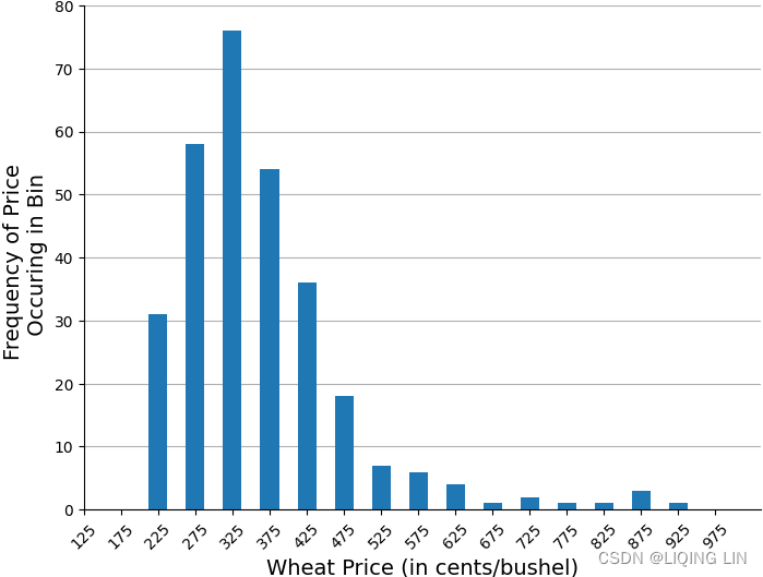
Now I want to shift the histogram or each bar to the right edge of the bin
OR show frequency distribution to the right tail
import matplotlib.pyplot as plt
import numpy as np

fig, ax = plt.subplots(1, figsize=(8,6),#gridspec_kw={'height_ratios': [2, 1]}
                      )
bin_width=50

hist_values, bin_edges= np.histogram( wheat['Wheat'],
                                      # it defines a monotonically increasing array of bin edges, including the rightmost edge
                                      bins=np.arange(0, 1000+bin_width, bin_width), # 21 bin_edges
                                      #range=( wheat['Wheat'].min(), wheat['Wheat'].max() ),
                                      density=False, # False: count the number of samples in each bin
                                    )
# len(hist_values), len(bin_edges) ==> (20 bins, 21 bin_edges)
# hist_values
# array([ 0,   0,   0,   0,  31,  58,  76,  54,  36,  18,
#         7,   6,   4,   1,   2,   1,   1,   3,   1,   0], dtype=int64)
# bin_edges
# array([ 0,  50, 100, 150, 200, 250, 300, 350, 400, 450,
#       500, 550, 600, 650, 700, 750, 800, 850, 900, 950,
#       1000])

#wheat.hist(column='Wheat(X)', bins=20, ax=ax)
ax.grid(axis='y', )
shift_hist=bin_width/2.0
ax.hist(x=bin_edges[1:], # use the right edges ########
        bins=bin_edges+shift_hist,             ########
        weights=hist_values,
        rwidth=0.5, # The relative width of the bars as a fraction of the bin width(here is 50)
        zorder=2.0,# set the grid line below the bar
        color='gray'
       )# bar_width = bin_width * rwidth = 50*0.5 = 25


#set the xticks with the middle position of bar = left edge + bar_width
ax.set_xticks(bin_edges[1:] ) # use the right edges ######
ax.set_xlim( left=100 )# set the start xtick

ax.set_xticklabels( ax.get_xticklabels(),
                    rotation=45
                  )

ax.set_yticks(np.arange(0,90, 10))
ax.set_xlabel('Wheat Price (in cents/bushel)', fontsize=14)
ax.set_ylabel('Frequency of Price \n Occuring in Bin', fontsize=14)

ax.spines['right'].set_visible(False)
ax.spines['top'].set_visible(False)
ax.spines['bottom'].set_color('gray')
ax.spines['left'].set_color('gray')
ax.tick_params(width=0) # Tick line width in points

plt.show()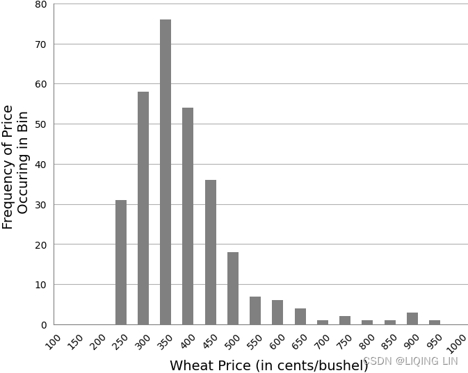
FIGURE 2.3 Wheat frequency distribution showing a tail to the right.
import matplotlib.pyplot as plt
import numpy as np

fig, ax = plt.subplots(1, figsize=(8,6),#gridspec_kw={'height_ratios': [2, 1]}
                      )
bin_width=50

hist_values, bin_edges= np.histogram( wheat['Wheat'],
                                      # it defines a monotonically increasing array of bin edges, including the rightmost edge
                                      bins=np.arange(0, 1000+bin_width, bin_width), # 21 bin_edges
                                      #range=( wheat['Wheat'].min(), wheat['Wheat'].max() ),
                                      density=False, # False: count the number of samples in each bin
                                    )
# len(hist_values), len(bin_edges) ==> (20 bins, 21 bin_edges)
# hist_values
# array([ 0,   0,   0,   0,  31,  58,  76,  54,  36,  18,
#         7,   6,   4,   1,   2,   1,   1,   3,   1,   0], dtype=int64)
# bin_edges
# array([ 0,  50, 100, 150, 200, 250, 300, 350, 400, 450,
#       500, 550, 600, 650, 700, 750, 800, 850, 900, 950,
#       1000])

#wheat.hist(column='Wheat(X)', bins=20, ax=ax)
#ax.grid(axis='y', )
shift_hist=bin_width/2.0
ax.hist(x=bin_edges[1:], # use the right edges ########
        bins=bin_edges+shift_hist,             ########
        weights=hist_values,
        rwidth=0.5, # The relative width of the bars as a fraction of the bin width(here is 50)
        zorder=2.0,# set the grid line below the bar
        color='gray'
       )# bar_width = bin_width * rwidth = 50*0.5 = 25


#set the xticks with the middle position of bar = left edge + bar_width
ax.set_xticks(bin_edges[1:] ) # use the right edges ######
ax.set_xlim( left=100 )# set the start xtick

ax.set_xticklabels( ax.get_xticklabels(),
                    rotation=45
                  )

ax.set_yticks([])
ax.set_xlabel('Wheat Price (in cents/bushel)', fontsize=14)
ax.set_ylabel('Frequency of Price \n Occuring in Bin', fontsize=14)

ax.spines['right'].set_visible(False)
ax.spines['top'].set_visible(False)
ax.spines['bottom'].set_color('gray')
ax.spines['left'].set_color('gray')
ax.tick_params(width=0) # Tick line width in points


label_n=1
for i,p in enumerate(ax.patches):
        x, w, h = p.get_x(), p.get_width(), p.get_height()

        if h > 0:
            count=hist_values[i]
            # https://matplotlib.org/stable/gallery/text_labels_and_annotations/text_alignment.html
            ax.text(x + w / 2, h, # the location(x + w/2, h) of the anchor point
                    f'{count}\n',
                    ha='center',  # center of text_box(square box) as the anchor point
                    va='center',  # center of text_box(square box) as the anchor point
                    size=7.5
                   )


plt.show()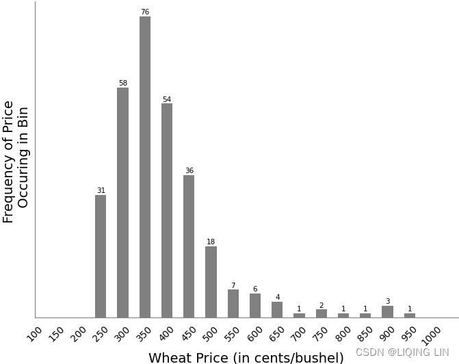
FIGURE 2.3 Wheat frequency distribution showing a tail to the right.
hist_values.sum()![]() vs
vs
import matplotlib.pyplot as plt
import numpy as np

fig, ax = plt.subplots(1, figsize=(8,6),#gridspec_kw={'height_ratios': [2, 1]}
                      )
bin_width=50

hist_values, bin_edges= np.histogram( wheat['Wheat'],
                                      # it defines a monotonically increasing array of bin edges, including the rightmost edge
                                      bins=np.arange(0, 1000+bin_width, bin_width), # 21 bin_edges
                                      #range=( wheat['Wheat'].min(), wheat['Wheat'].max() ),
                                      density=False, # False: count the number of samples in each bin
                                    )
# len(hist_values), len(bin_edges) ==> (20 bins, 21 bin_edges)
# hist_values
# array([ 0,   0,   0,   0,  31,  58,  76,  54,  36,  18,
#         7,   6,   4,   1,   2,   1,   1,   3,   1,   0], dtype=int64)
# bin_edges
# array([ 0,  50, 100, 150, 200, 250, 300, 350, 400, 450,
#       500, 550, 600, 650, 700, 750, 800, 850, 900, 950,
#       1000])

#wheat.hist(column='Wheat(X)', bins=20, ax=ax)
#ax.grid(axis='y', )
shift_hist=bin_width/2.0
ax.hist(x=bin_edges[1:], # use the right edges ########
        bins=bin_edges+shift_hist,             ########
        weights=hist_values,
        rwidth=0.5, # The relative width of the bars as a fraction of the bin width(here is 50)
        zorder=2.0,# set the grid line below the bar
        color='gray'
       )# bar_width = bin_width * rwidth = 50*0.5 = 25


#set the xticks with the middle position of bar = left edge + bar_width
ax.set_xticks(bin_edges[1:] ) # use the right edges ######
ax.set_xlim( left=100 )# set the start xtick

ax.set_xticklabels( ax.get_xticklabels(),
                    rotation=45
                  )

ax.set_yticks([])
ax.set_xlabel('Wheat Price (in cents/bushel)', fontsize=14)
ax.set_ylabel('Frequency of Price \n Occuring in Bin', fontsize=14)

ax.spines['right'].set_visible(False)
ax.spines['top'].set_visible(False)
ax.spines['bottom'].set_color('gray')
ax.spines['left'].set_color('gray')
ax.tick_params(width=0) # Tick line width in points


label_n=1
for p in ax.patches:
        x, w, h = p.get_x(), p.get_width(), p.get_height()

        if h > 0:
            pct=h / len(wheat['Wheat'])
            # https://matplotlib.org/stable/gallery/text_labels_and_annotations/text_alignment.html
            ax.text(x + w / 2, h, # the location(x + w/2, h) of the anchor point
                    f'{pct*100:.2f}%\n',
                    ha='center',  # center of text_box(square box) as the anchor point
                    va='center',  # center of text_box(square box) as the anchor point
                    size=7.5
                   )

plt.show()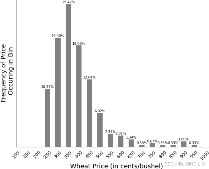
When completed, you will have 20 bins that begin at the lowest price and end at the highest price. You then can count the number of prices that fall into each bin, a nearly impossible task, or you can use a spreadsheet to do it. In Excel, you go to Data/Data Analysis/Histogram and enter the range of bins (which you need to set up in advance) and the data to be analyzed, then select a blank place on the spreadsheet for the output results (to the right of the bins is good) and click OK. The frequency distribution will be shown instantly. You can then plot the results seen in Figure 2.3.
The frequency distribution shows that the most common price fell between $3.50 and $4.00 per bushel (check the following normal distributin plot)but the most active range was from $2.50 to $5.00. The tail to the right extends to just under $10/bushel and clearly demonstrates the fat tail in the price distribution. If this was a normal distribution, there would be no entries past $6.0(based on 95% confidence interval).
numpy.histogram(a, bins=10, range=None, density=None, weights=None)
density bool, optional
If False, the result will contain the number of samples in each bin.
If True, the result is the value of the Probability Density Function at the bin, normalized such that the integral over the range is 1. Note that the sum of the histogram values will not be equal to 1 unless bins of unity width are chosen; it is not a probability mass function.请注意,直方图值的总和将不等于 1,除非选择单位宽度的 bin(对数据进行z-score![]() transformationts8_Outlier Detection_plotly_sns_text annot_modified z-score_hist_Tukey box_cdf_resample freq_Quanti_LIQING LIN的博客-CSDN博客
transformationts8_Outlier Detection_plotly_sns_text annot_modified z-score_hist_Tukey box_cdf_resample freq_Quanti_LIQING LIN的博客-CSDN博客
Notice how the shape of the data did not change, hence why the z-score is called a lossless transformation. The only difference between the two is the scale (units).
); 它不是概率质量函数。
import matplotlib.pyplot as plt
import numpy as np
from scipy.stats import norm

fig, ax = plt.subplots(1, figsize=(8,6),#gridspec_kw={'height_ratios': [2, 1]}
                      )


bin_width=50

hist_values, bin_edges= np.histogram( wheat['Wheat'],
                                      # it defines a monotonically increasing array of bin edges, including the rightmost edge
                                      bins=np.arange(0, 1000+bin_width, bin_width), # 21 bin_edges
                                      #range=( wheat['Wheat'].min(), wheat['Wheat'].max() ),
                                      density=True, # False: count the number of samples in each bin
                                    )
# len(hist_values), len(bin_edges) ==> (20 bins, 21 bin_edges)
# hist_values
# array([ 0,   0,   0,   0,  31,  58,  76,  54,  36,  18,
#         7,   6,   4,   1,   2,   1,   1,   3,   1,   0], dtype=int64)
# bin_edges
# array([ 0,  50, 100, 150, 200, 250, 300, 350, 400, 450,
#       500, 550, 600, 650, 700, 750, 800, 850, 900, 950,
#       1000])

#wheat.hist(column='Wheat(X)', bins=20, ax=ax)
#ax.grid(axis='y', )
shift_hist=bin_width/2.0
ax.hist(x=bin_edges[:-1], # use the left edges
        bins=bin_edges,
        weights=hist_values,
        rwidth=1, # The relative width of the bars as a fraction of the bin width(here is 50)
        zorder=2.0,# set the grid line below the bar
        ec="black"
       )# bar_width = bin_width * rwidth = 50*0.5 = 25

#set the xticks with the middle position of bar = left edge + bar_width
ax.set_xticks(bin_edges )
ax.set_xlim( left=0 )# set the start xtick

ax.set_xticklabels( ax.get_xticklabels(),
                    rotation=45
                  )

# Fit a normal distribution to
# the data:
# mean and standard deviation
mu, std = norm.fit(wheat['Wheat'])
# mu, std : (362.7483277591973, 115.83166808628707)

# Plot the PDF.
# mu, std = wheat['Wheat'].mean(), wheat['Wheat'].std()
# (362.7483277591973, 116.02585375167453)

x = np.linspace(0, #start
                1000, #stop
                100#Number of samples to generate
               )
p = norm.pdf(x, mu, std)
r_min = norm.ppf(0.025, mu, std)   #
r_max = norm.ppf(1-0.025, mu, std) #

ax.plot(x, #since we shift all bars to the right edge
        p, 'blue', linewidth=2, zorder=3.0)
plt.fill_between(x, p, 0, where= (x<r_min),color='orange',zorder=3.0 )
plt.fill_between(x, p, 0, where= (r_max<x),color='orange',zorder=3.0 )

ax.set_yticks([])
ax.set_xlabel('Wheat Price (in cents/bushel)', fontsize=14)
ax.set_ylabel('Probability Density Function', fontsize=14, color='blue')

ax.spines['right'].set_visible(False)
ax.spines['top'].set_visible(False)
ax.spines['bottom'].set_color('gray')
ax.spines['left'].set_color('gray')
ax.tick_params(width=0) # Tick line width in points

plt.show()
import matplotlib.pyplot as plt
import numpy as np
from scipy.stats import norm

fig, ax = plt.subplots(1, figsize=(8,6),#gridspec_kw={'height_ratios': [2, 1]}
                      )


bin_width=50

hist_values, bin_edges= np.histogram( wheat['Wheat'],
                                      # it defines a monotonically increasing array of bin edges, including the rightmost edge
                                      bins=np.arange(0, 1000+bin_width, bin_width), # 21 bin_edges
                                      #range=( wheat['Wheat'].min(), wheat['Wheat'].max() ),
                                      density=True, # False: count the number of samples in each bin
                                    )
# len(hist_values), len(bin_edges) ==> (20 bins, 21 bin_edges)
# hist_values
# array([ 0,   0,   0,   0,  31,  58,  76,  54,  36,  18,
#         7,   6,   4,   1,   2,   1,   1,   3,   1,   0], dtype=int64)
# bin_edges
# array([ 0,  50, 100, 150, 200, 250, 300, 350, 400, 450,
#       500, 550, 600, 650, 700, 750, 800, 850, 900, 950,
#       1000])

#wheat.hist(column='Wheat(X)', bins=20, ax=ax)
#ax.grid(axis='y', )
shift_hist=bin_width/2.0
ax.hist(x=bin_edges[:-1], # use the left edges
        bins=bin_edges,
        weights=hist_values,
        rwidth=1, # The relative width of the bars as a fraction of the bin width(here is 50)
        zorder=2.0,# set the grid line below the bar
        ec="black"
       )# bar_width = bin_width * rwidth = 50*0.5 = 25

#set the xticks with the middle position of bar = left edge + bar_width
ax.set_xticks(bin_edges )
ax.set_xlim( left=100 )# set the start xtick

ax.set_xticklabels( ax.get_xticklabels(),
                    rotation=45
                  )

# Fit a normal distribution to
# the data:
# mean and standard deviation
mu, std = norm.fit(wheat['Wheat'])
# mu, std : (362.7483277591973, 115.83166808628707)

# Plot the PDF.
# mu, std = wheat['Wheat'].mean(), wheat['Wheat'].std()
# (362.7483277591973, 116.02585375167453)

x = np.linspace(mu-2*std, # 95% confidence interval
                mu+2*std,
                100
               )
p = norm.pdf(x, mu, std)

ax.plot(x, #since we shift all bars to the right edge
        p, 'blue', linewidth=2, zorder=3.0)

#ax.set_yticks([])
ax.set_xlabel('Wheat Price (in cents/bushel)', fontsize=14)
ax.set_ylabel('Probability Density Function', fontsize=14, color='blue')

ax.spines['right'].set_visible(False)
ax.spines['top'].set_visible(False)
ax.spines['bottom'].set_color('gray')
ax.spines['left'].set_color('gray')
ax.tick_params(width=0) # Tick line width in points

plt.show()
the area under the black line : 95% confidence interval

FIGURE 2.4 Normal distribution showing the percentage area included within one standard deviation about the arithmetic mean.
import matplotlib.pyplot as plt
import numpy as np
from scipy.stats import norm

fig, ax = plt.subplots(1, figsize=(8,6),#gridspec_kw={'height_ratios': [2, 1]}
                      )


bin_width=50

hist_values, bin_edges= np.histogram( wheat['Wheat'],
                                      # it defines a monotonically increasing array of bin edges, including the rightmost edge
                                      bins=np.arange(0, 1000+bin_width, bin_width), # 21 bin_edges
                                      #range=( wheat['Wheat'].min(), wheat['Wheat'].max() ),
                                      density=True, # False: count the number of samples in each bin
                                    )
# len(hist_values), len(bin_edges) ==> (20 bins, 21 bin_edges)
# hist_values
# array([ 0,   0,   0,   0,  31,  58,  76,  54,  36,  18,
#         7,   6,   4,   1,   2,   1,   1,   3,   1,   0], dtype=int64)
# bin_edges
# array([ 0,  50, 100, 150, 200, 250, 300, 350, 400, 450,
#       500, 550, 600, 650, 700, 750, 800, 850, 900, 950,
#       1000])

#wheat.hist(column='Wheat(X)', bins=20, ax=ax)
#ax.grid(axis='y', )
shift_hist=bin_width/2.0
ax.hist(x=bin_edges[:-1], # use the left edges
        bins=bin_edges,
        weights=hist_values,
        rwidth=0.5, # The relative width of the bars as a fraction of the bin width(here is 50)
        zorder=2.0,# set the grid line below the bar
       )# bar_width = bin_width * rwidth = 50*0.5 = 25

#set the xticks with the middle position of bar = left edge + bar_width
ax.set_xticks(bin_edges[:-1]+bin_width/2. ) # with the value of the middle position on each bin
ax.set_xlim( left=100+bin_width/2. )# set the start xtick

ax.set_xticklabels( ax.get_xticklabels(),
                    rotation=45
                  )

# Fit a normal distribution to
# the data:
# mean and standard deviation
mu, std = norm.fit(wheat['Wheat'])
# mu, std : (362.7483277591973, 115.83166808628707)

# Plot the PDF.
# mu, std = wheat['Wheat'].mean(), wheat['Wheat'].std()
# (362.7483277591973, 116.02585375167453)

x = np.linspace(mu-2*std, # 95% confidence interval
                mu+2*std,
                100
               )
p = norm.pdf(x, mu, std)

ax.plot(x, #since we shift all bars to the right edge
        p, 'k', linewidth=2, zorder=3.0)

#ax.set_yticks([])
ax.set_xlabel('Wheat Price (in cents/bushel)', fontsize=14)
ax.set_ylabel('Probability Density Function', fontsize=14)

ax.spines['right'].set_visible(False)
ax.spines['top'].set_visible(False)
ax.spines['bottom'].set_color('gray')
ax.spines['left'].set_color('gray')
ax.tick_params(width=0) # Tick line width in points

plt.show()
import matplotlib.pyplot as plt
import numpy as np
from scipy.stats import norm

fig, ax = plt.subplots(1, figsize=(8,6),#gridspec_kw={'height_ratios': [2, 1]}
                      )


bin_width=50

hist_values, bin_edges= np.histogram( wheat['Wheat'],
                                      # it defines a monotonically increasing array of bin edges, including the rightmost edge
                                      bins=np.arange(0, 1000+bin_width, bin_width), # 21 bin_edges
                                      #range=( wheat['Wheat'].min(), wheat['Wheat'].max() ),
                                      density=True, # False: count the number of samples in each bin
                                    )
# len(hist_values), len(bin_edges) ==> (20 bins, 21 bin_edges)
# hist_values
# array([ 0,   0,   0,   0,  31,  58,  76,  54,  36,  18,
#         7,   6,   4,   1,   2,   1,   1,   3,   1,   0], dtype=int64)
# bin_edges
# array([ 0,  50, 100, 150, 200, 250, 300, 350, 400, 450,
#       500, 550, 600, 650, 700, 750, 800, 850, 900, 950,
#       1000])

#wheat.hist(column='Wheat(X)', bins=20, ax=ax)
#ax.grid(axis='y', )
shift_hist=bin_width/2.0
ax.hist(x=bin_edges[1:], # use the right edges ########
        bins=bin_edges+shift_hist,             ########
        weights=hist_values,
        rwidth=0.5, # The relative width of the bars as a fraction of the bin width(here is 50)
        zorder=2.0,# set the grid line below the bar
        color='gray'
       )# bar_width = bin_width * rwidth = 50*0.5 = 25

#set the xticks with the middle position of bar = left edge + bar_width
ax.set_xticks(bin_edges[1:] ) # use the right edges ######
ax.set_xlim( left=100 )# set the start xtick

ax.set_xticklabels( ax.get_xticklabels(),
                    rotation=45
                  )

# Fit a normal distribution to
# the data:
# mean and standard deviation
mu, std = norm.fit(wheat['Wheat'])
# mu, std : (362.7483277591973, 115.83166808628707)

# Plot the PDF.
# mu, std = wheat['Wheat'].mean(), wheat['Wheat'].std()
# (362.7483277591973, 116.02585375167453)

x = np.linspace(mu-2*std, # 95% confidence interval
                mu+2*std,
                100
               )
p = norm.pdf(x, mu, std)

ax.plot(x, #since we shift all bars to the right edge
        p, 'k', linewidth=2, zorder=3.0)

ax.set_yticks([])
ax.set_xlabel('Wheat Price (in cents/bushel)', fontsize=14)
ax.set_ylabel('Probability Density Function', fontsize=14)

ax.spines['right'].set_visible(False)
ax.spines['top'].set_visible(False)
ax.spines['bottom'].set_color('gray')
ax.spines['left'].set_color('gray')
ax.tick_params(width=0) # Tick line width in points

plt.show()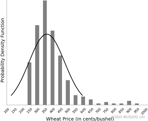
The absence of price data below $2.50 is due to the cost of production. Below that price farmers would refuse to sell at a loss; however, the U.S. government has a price support program that guarantees a minimum return for farmers.
The wheat frequency distribution can also be viewed net of inflation or changes in the U.S. dollar(扣除通货膨胀或美元变化后). This will be seen at the end of this chapter
The same frequency distributions occur even when we look at shorter time intervals, although the pattern is more erratic as the time interval gets very small. If we take wheat prices for the calendar year 2007 (Figure 2.4) we see a steady move up during midyear年中, followed by a wide-ranging sideways pattern at higher level;
# https://www.macrotrends.net/2534/wheat-prices-historical-chart-data
wheat40 = pd.read_csv('wheat-prices-historical-chart-data.csv',
                       index_col=0,
                       skiprows=16,
                       names=['Date','Wheat']
                      )[:'2023-01-01']
# #wheat40['2007-01-01':'2008-01-01']
# #Calculates the log returns
wheat40['log_rtn'] = np.log( wheat40['Wheat']/wheat40['Wheat'].shift(1) )
wheat40['Wheat(X)']=100

# # estimated future price = (log return * 100) + previous price
for i in range(1,len(wheat40)):
        wheat40.iloc[i,
                     list(wheat40.columns).index( 'Wheat(X)' )
                    ]= wheat40['Wheat(X)'].iloc[i-1] + 100*wheat40['log_rtn'].iloc[i]
#wheat['Wheat(X)'][0]=100
wheat40['2007-01-01':'2008-01-01']
wheat40['2007-01-01':'2008-01-01']['Wheat'].plot()
plt.show()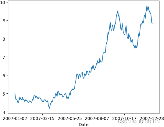
FIGURE 2.4 Wheat daily prices, 2007.
however, the frequency distribution in Figure 2.5 shows a pattern similar to the long-term distribution, with the most common value at a low price level and a fat tail to the right.
import matplotlib.pyplot as plt
import numpy as np
from scipy.stats import norm

fig, ax = plt.subplots(1, figsize=(8,6),#gridspec_kw={'height_ratios': [2, 1]}
                      )


bin_width=50

hist_values, bin_edges= np.histogram( wheat40['2007-01-01':'2008-01-01']['Wheat']*100,
                                      # it defines a monotonically increasing array of bin edges, including the rightmost edge
                                      bins=np.arange(0, 1000+bin_width, bin_width), # 21 bin_edges
                                      #range=( wheat['Wheat'].min(), wheat['Wheat'].max() ),
                                      density=True, # False: count the number of samples in each bin
                                    )
# len(hist_values), len(bin_edges) ==> (20 bins, 21 bin_edges)
# hist_values
# array([ 0,   0,   0,   0,  31,  58,  76,  54,  36,  18,
#         7,   6,   4,   1,   2,   1,   1,   3,   1,   0], dtype=int64)
# bin_edges
# array([ 0,  50, 100, 150, 200, 250, 300, 350, 400, 450,
#       500, 550, 600, 650, 700, 750, 800, 850, 900, 950,
#       1000])

#wheat.hist(column='Wheat(X)', bins=20, ax=ax)
#ax.grid(axis='y', )
shift_hist=bin_width/2.0
ax.hist(x=bin_edges[1:], # use the right edges ########
        bins=bin_edges+shift_hist,             ########
        weights=hist_values,
        rwidth=0.5, # The relative width of the bars as a fraction of the bin width(here is 50)
        zorder=2.0,# set the grid line below the bar
        color='gray'
       )# bar_width = bin_width * rwidth = 50*0.5 = 25

#set the xticks with the middle position of bar = left edge + bar_width
ax.set_xticks(bin_edges[1:] ) # use the right edges ######
ax.set_xlim( left=400 )# set the start xtick

ax.set_xticklabels( ax.get_xticklabels(),
                    rotation=45
                  )

# Fit a normal distribution to
# the data:
# mean and standard deviation
mu, std = norm.fit(wheat40['2007-01-01':'2008-01-01']['Wheat']*100)
# mu, std : (362.7483277591973, 115.83166808628707)

# Plot the PDF.
# mu, std = wheat['Wheat'].mean(), wheat['Wheat'].std()
# (362.7483277591973, 116.02585375167453)

x = np.linspace(mu-2*std, # 95% confidence interval
                mu+2*std,
                100
               )
p = norm.pdf(x, mu, std)

ax.plot(x, #since we shift all bars to the right edge
        p, 'k', linewidth=2, zorder=3.0)

ax.set_yticks([])
ax.set_xlabel('Wheat Price (in dollars/bushel)', fontsize=14)
ax.set_ylabel('Probability Density Function', fontsize=14)

ax.spines['right'].set_visible(False)
ax.spines['top'].set_visible(False)
ax.spines['bottom'].set_color('gray')
ax.spines['left'].set_color('gray')
ax.tick_params(width=0) # Tick line width in points

plt.show()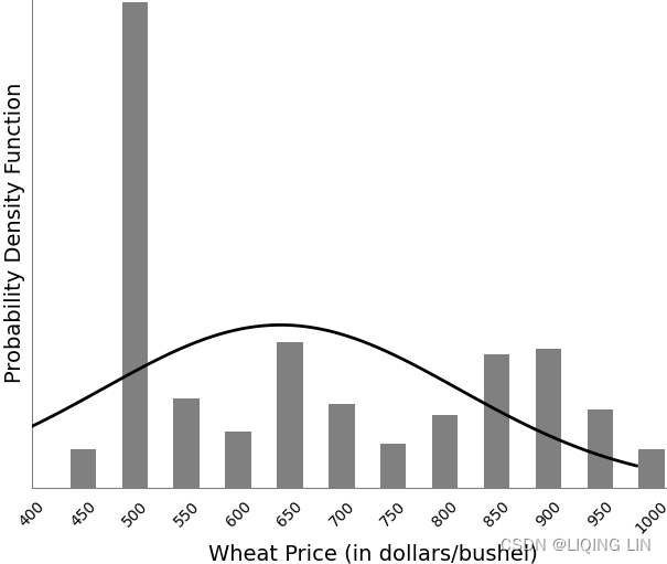
FIGURE 2.5 Frequency distribution of wheat prices, intervals of $0.50, during 2007.
If we had picked the few months just before prices peaked in September 2007, the chart might have shown the peak price further to the right and the fat tail on the left. For commodities, this represents a period of price instability, and expectations that prices will fall.


 It should be expected that the distribution of prices for a physical commodity, such as agricultural products, metals, and energy will be skewed toward the left (more occurrences at lower prices) and have a long tail at higher prices toward the right of the chart.应该预料到,农产品、金属和能源等实物商品的价格分布将向左倾斜(价格越低出现次数越多),并且在图表右侧的价格较高时有一条长尾巴 This is because prices remain at relatively higher levels for only short periods of time while there is an imbalance in supply and demand.
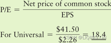
In the stock market, history has shown that stocks will not sustain exceptionally high price/earnings (P/E) ratios indefinitely; however, the period of adjustment can be drawn out over many years, unlike an agricultural product that begins again each year. When observing shorter price periods, patterns that do not fit the standard distribution may be considered in transition. Readers who would like to pursue this topic should read Chapter 18, especially the sections “Distribution of Prices” and “Steidlmayer’s Market Profile.”
The measures of central tendency discussed in the previous section are used to describe the shape and extremes of price movement shown in the frequency distribution. The general relationship between the three principal means when the distribution is not perfectly symmetric is 当分布不完全对称时,三个主要均值之间的一般关系是
#1_Statistics_agent_policy_explanatory_predictor_response_numeric_mode_Hypothesis_Type I_Chi-squ_LIQING LIN的博客-CSDN博客Median(==Q2, the second quartile): This is the midpoint of the data, and is calculated by either arranging it in ascending or descending order. If there are N observations.
Application: Binary search or students' score(if the average(mean)>60, and your professor want at least half of students pass the course, but if your professor use the mean as measure, then most number of students will fail since few students got very high score and the mean is affected by the high scores(this means the average will not reflect the “typically” student scores), so he will consider to use the median of the scores as measure)
Find the median of a batch of n numbers is easy as long as you remember to order the values first.
If n is odd, the median is the middle value. Counting in from the ends, we find the value in the (n+1)/2 position
if n is even, there are two middle values. So, in the case, the median is the average of the two values in positions n/2 and n/2+1


Two other measurements, the median and the mode, are often used to define distribution. The median, or “middle item,” is helpful for establishing the “center” of the data; when the data is sorted, it is the value in the middle. The median has the advantage of discounting extreme values中位数的优点是可以忽略极值, which might distort the arithmetic mean极值可能会扭曲算术平均值. Its disadvantage is that you must sort all of the data in order to locate the middle point. The median is preferred over the mean except when using a very small number of items.
The mode is the most commonly occurring value. In Figure 2.5, the mode is the highest bar in the frequency distribution, at bin 500.
In a normally distributed price series, the mode, mean, and median all occur at the same value; however, as the data becomes skewed, these values will move farther apart. The general relationship is: Mode < Median < Mean (positively skewed)
Mean < Median < Mode (negatively skewed)
A normal distribution is commonly called a bell curve, and values fall equally on both sides of the mean. For much of the work done with price and performance data, the distributions tend to be skewed to the right (Mode < Median < Mean: toward higher prices or higher trading profits), and appear to flatten or cut off on the left (lower prices or trading losses). If you were to chart a distribution of trading profits and losses based on a trend system with a fixed stop-loss, you would get profits that could range from zero to very large values, while the losses would be theoretically limited to the size of the stop-loss如果您要根据具有固定止损的趋势系统绘制交易利润和损失的分布图,您将获得从零到非常大的值的利润,而损失在理论上将限制在止损的大小. Skewed distributions will be important when we measure probabilities later in this chapter. There are no “normal” distributions in a trading environment.
Each averaging method has its unique meaning and usefulness. The following summary points out their principal characteristics:
==>is most applicable to time changes and, along with the geometric mean, has been used in economics for price analysis. It is more difficult to calculate; therefore, it is less popular than either of the other averages, although it is also capable of algebraic manipulation.The moments of the distribution describe the shape of the data points, which is the way they cluster around the mean. There are four moments: mean, variance, skew, and kurtosis, each describing a different aspect of the shape of the distribution. Simply put, the mean is the center or average value, the variance is the distance of the individual points from the mean, the skew is the way the distribution leans to the left or right relative to the mean, and the kurtosis is the peakedness of the clustering. We have already discussed the mean, so we will start with the 2nd moment.
In the following calculations, we will use the bar notation, ![]() , to indicate the average of a list of n prices. The capital P refers to all prices and the small P to individual prices.
, to indicate the average of a list of n prices. The capital P refers to all prices and the small P to individual prices.
The Mean Deviation (MD) is a basic method for measuring distribution and may be calculated about any measure of central location, such as the arithmetic mean.
Then MD is the average of the differences between each price and the arithmetic mean of those prices, or some other measure of central location, with all differences treated as positive numbers.
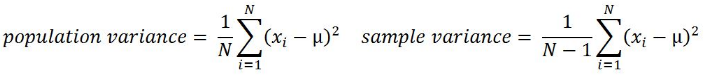
Variance (Var), which is very similar to mean deviation, the best estimation of dispersion/dɪˈspɜːrʒn/分布, will be used as the basis for many other calculations. It is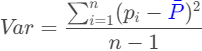
This is the mean of squared deviations from the mean ( = data points, µ = mean of the data, N = number of data points). The dimension of variance is the square of the actual values. The reason to use denominator N-1 for a sample instead of N in the population is due the degree of freedom. 1 degree of freedom lost in a sample by the time of calculating variance is due to extraction of substitution of sample:


Notice that the variance is the square of the standard deviation, ![]() , one of the most commonly used statistics. In Excel, the variance is the function var(list).
, one of the most commonly used statistics. In Excel, the variance is the function var(list).
The standard deviation (s), most often shown as (sigma), is a special form of σ measuring average deviation from the mean, which uses the root-mean-square
where the differences between the individual prices and the mean are squared to emphasize the significance of extreme values, and then the total value is scaled back using the square root function. The standard deviation is the square root of variance. By applying the square root on variance, we measure the dispersion with respect to the original variable rather than square of the dimension:
The standard deviation is the most popular way of measuring the dispersion of data.
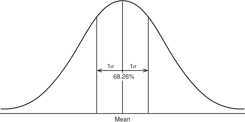 FIGURE 2.6 Normal distribution showing the percentage area included within one standard deviation about the arithmetic mean.
 (3)
(3)
Most price data, however, are not normally distributed. For physical commodities, such as gold, grains, energy, and even interest rates (expressed at yields以收益率表示), prices tend to spend more time at low levels and much less time at extreme highs( physical commodity, such as agricultural products, metals, and energy will be skewed toward the left (more occurrences at lower prices) and have a long tail at higher prices toward the right of the chart). While gold peaked at $800 per ounce for one day in January 1980, it remained between $250 and $400 per ounce for most of the next 20 years. If we had taken the average at $325 then is would be impossible for the price distribution to be symmetric. If 1 standard deviation is $140, then a normal distribution would show a high likelihood of prices dropping to $185(325-140=185), an unlikely scenario. This asymmetry is most obvious in agricultural markets, where a shortage of soybeans or coffee in one year will drive prices much higher, but a normal crop the following year will return those prices to previous levels.
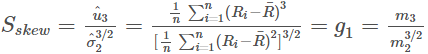
The relationship of price versus time, where markets spend more time at lower levels, can be measured as skewness—the amount of distortion from a symmetric distribution, which makes the curve appear to be short on the left and extended to the right (higher prices). The extended side is called the tail, and a longer tail to the right is called positive skewness. Negative skewness has the tail extending toward the left. This can be seen in Figure 2.7. 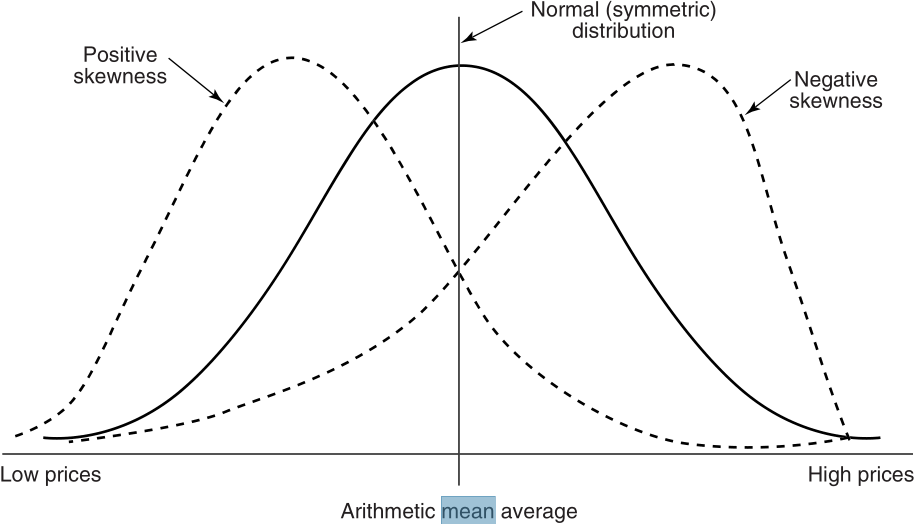 FIGURE 2.7 Skewness. Nearly all price distributions are positively skewed, showing a longer tail to the right, at higher prices.
In a perfectly normal distribution, the mean, median, and mode all coincide. As prices become positively skewed,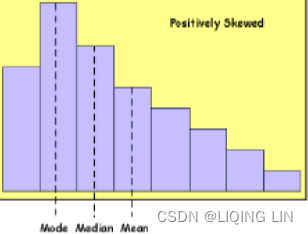 typical of a period of higher prices, the mean will show the greatest change, the mode will show the least, and the median will fall in between. The difference between the mean and the mode, adjusted for dispersion using the standard deviation of the distribution使用分布的标准偏差 针对 离差进行调整, gives a good measure of skewness.
 ![]()
The distance between the mean and the mode, in a moderately skewed distribution适度偏态分布, turns out to be three times the difference between the mean and the median; the relationship can also be written as:![]()
To show the similarity between the 2nd and 3rd moments (variance and skewness) the more common computational formula is(The sample skewness is computed as the Fisher-Pearson coefficient of skewness, i.e.)
(3) is the biased sample mth central moment
The skewness of a data series can sometimes be corrected using a transformation. Price data may be skewed in a specific pattern. For example, if there are 3 occurrences at twice the price, and 1/9 of the occurrences at 3 times the price, this may result in a positively skewed distribution(如果价格数据的模式是价格的两倍出现 3 次,价格的三倍出现 1/9,这可能会导致正偏分布). In this case, taking the square root of each data item can transform the data into a normal distribution. The characteristics of price data often show a logarithmic, power, or square-root relationship. For example,
ibm_df['log_rtn'] = np.log( ibm_df['Adj Close']/ibm_df['Adj Close'].shift(1) )
from scipy.stats import shapiro, kstest, normaltest
from statsmodels.stats.diagnostic import kstest_normal, normal_ad

def is_normal( test, p_level=0.05, name='' ):
    stat, pvalue = test
    print( name + ' test')
    print( 'statistic: ', stat )
    print( 'p-value:', pvalue)
    return 'Normal' if pvalue>0.05 else 'Not Normal'

normal_args = ( np.mean(ibm_df['sim_rtn'].dropna()), np.std(ibm_df['sim_rtn'].dropna()) )

# The Shapiro-Wilk test tests the null hypothesis that
# the data was drawn from a normal distribution.
print( is_normal( shapiro(ibm_df['sim_rtn'].dropna()), name='##### Shapiro-Wilk' ) )

# Test whether a sample differs from a normal distribution.
# statistic:                     z-score = (x-mean)/std
#           s^2 + k^2, where s is the z-score returned by skewtest
#           and k is the z-score returned by kurtosistest.
print( is_normal( normaltest(ibm_df['sim_rtn'].dropna()), name='##### normaltest' ) )

# Anderson-Darling test for normal distribution unknown mean and variance.
print( is_normal( normal_ad(ibm_df['sim_rtn'].dropna()), name='##### Anderson-Darling' ) )

# Test assumed normal or exponential distribution using Lilliefors’ test.
# Kolmogorov-Smirnov test statistic with estimated mean and variance.
print( is_normal( kstest_normal(ibm_df['sim_rtn'].dropna()), name='##### Kolmogorov-Smirnov') )

# The one-sample test compares the underlying distribution F(x) of
# a sample against a given distribution G(x).
# The two-sample test compares the underlying distributions of
# two independent samples.
# Both tests are valid only for continuous distributions.
print( is_normal( kstest( ibm_df['sim_rtn'].dropna(),
                          cdf='norm',
                          args=normal_args
                        ), name='##### KS'
                )
     )
# https://blog.csdn.net/Linli522362242/article/details/128294150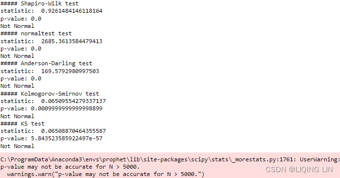
The output from the tests confirms the data does not come from a normal distribution. You do not need to run that many tests. The shapiro test, for example, is a very common and popular test that you can rely on.
To calculate the probability level of a distribution based on the skewed distribution of price, we can convert the normal probability to the exponential probability equivalent, ![]() , using要计算基于价格偏态分布的 分布的概率水平,我们可以将正态概率转换为等价的指数概率
, using要计算基于价格偏态分布的 分布的概率水平,我们可以将正态概率转换为等价的指数概率 

FIGURE 2.7 Skewness. Nearly all price distributions are positively skewed, showing a longer tail to the right, at higher prices.
Because the lower price levels of most commodities are determined by production costs, price distributions show a clear tendency to resist moving below these thresholds. This contributes to the positive skewness in those markets. Considering only the short term, when prices are at unusually high levels, they can be volatile and unstable, causing a negative skewness that can be interpreted as being top heavy. Somewhere between the very high and very low price levels, we may find a frequency distribution that looks normal. Figure 2.8 shows the change in the distribution of prices over, for example, 20 days as prices move sharply higher图 2.8 显示了价格分布在例如 20 天内随着价格急剧上涨而发生的变化. The mean shows the center of the distributions as they change from positive to negative skewness. This pattern indicates that a normal distribution is not appropriate for all price analysis, and that a log, exponential, or power distribution would only apply best to long-term analysis.此模式表明正态分布并不适合所有价格分析,对数分布、指数分布或幂分布仅最适用于长期分析。
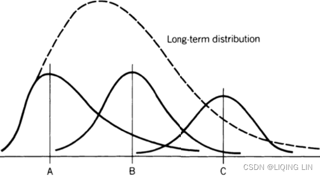
FIGURE 2.8 Changing distribution at different price levels. A, B, and C are increasing mean values of three shorter-term distributions and show the distribution changing from positive to negative skewness.
One last measurement, kurtosis, is needed to describe the shape of a price distribution. Kurtosis is the peakedness or flatness of a distribution as shown in Figure 2.9. This measurement is good for an unbiased assessment of whether prices are trending or moving sideways.
Steidlmayer’s Market Profile, discussed in Chapter 18, uses the concept of kurtosis, with the frequency distribution accumulated dynamically using real-time price changes频率分布使用实时价格变化动态累积.
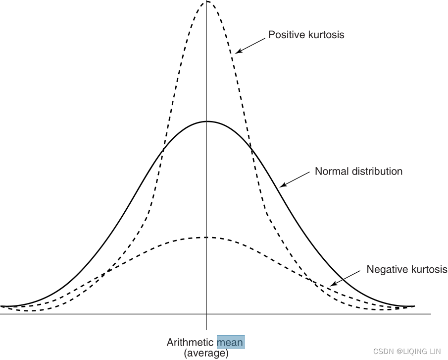
FIGURE 2.9 Kurtosis. A positive kurtosis is when the peak of the distribution is greater than normal, typical of a sideways market. A negative kurtosis, shown as a flatter distribution, occurs when the market is trending.
Following the same form as the 3rd moment, skewness, kurtosis can be calculated as
The kurtosis refects the impact of extreme values because of its power of four. There are two types of definitions with and without minus three; refer to the following two equations. The reason behind the deduction of three in equation (4B), is that for a normal distribution, its kurtosis based on equation (4A) is three(对于正态分布,基于等式 (4A) 的峰度为三):
https://blog.csdn.net/Linli522362242/article/details/128294150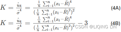 总体超峰度的有偏估计量
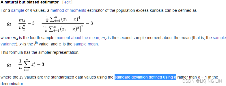
data standardization is a process of converting data to z-score values![]() based on the mean and standard deviation of the data
based on the mean and standard deviation of the data
scipy.stats.kurtosis(a, axis=0, fisher=True, bias=True, nan_policy='propagate', *, keepdims=False)
fisher bool, optional
Some books distinguish these two equations by calling equation (4B) excess kurtosis超峰度. However, many functions based on equation (4B) are still named kurtosis. Since we know that a standard normal distribution has a zero mean, unit standard deviation, zero skewness(为方便计算,将峰度值-3 ( Kurtosis-3 ),因此正态分布的峰度变为0,方便比较。), and zero kurtosis (based on equation 4B).
An alternative calculation for kurtosis is
Standard unbiased estimator
Given a sub-set of samples from a population, the sample excess kurtosis ![]() above is a biased estimator of the population excess kurtosis. An alternative estimator of the population excess kurtosis, which is unbiased in random samples of a normal distribution, is defined as follows
above is a biased estimator of the population excess kurtosis. An alternative estimator of the population excess kurtosis, which is unbiased in random samples of a normal distribution, is defined as follows 

其中k4是第四个累积量的唯一对称无偏估计,k2是第二个累积量(cumulant)的无偏估计(与样本方差的无偏估计相同),m4是关于均值的第四个样本矩,m2是第二个样本矩 关于均值,xi 是第 i 个值,并且![]() 是样本均值。 调整后的 Fisher-Pearson 标准化力矩系数
是样本均值。 调整后的 Fisher-Pearson 标准化力矩系数![]() 是在 Excel 和几个统计软件包(包括 Minitab、SAS 和 SPSS)中找到的版本。
是在 Excel 和几个统计软件包(包括 Minitab、SAS 和 SPSS)中找到的版本。
不幸的是,在非正态样本中![]() 本身通常是有偏见的。
本身通常是有偏见的。
Most often the excess kurtosis is used, which makes it easier to see abnormal distributions. Excess kurtosis, KE = K – 3 because the normal value of the kurtosis is 3 (为方便计算,将峰度值-3 ( Kurtosis-3 ),因此正态分布的峰度变为0,方便比较。).
Kurtosis is also useful when reviewing system tests. If you find the kurtosis of the daily returns, they should be somewhat better than normal if the system is profitable; however, if the kurtosis is above 7 or 8, then it begins to look as though the trading method is overfitted. A high kurtosis means that there are an overwhelming number of profitable trades of similar size, which is not likely to happen in real trading. Any high value of kurtosis should make you immediately suspicious. 峰态在审查系统测试时也很有用。 如果您发现每日收益的峰度,如果系统有利可图,它们应该比正常情况好一些; 但是,如果峰度高于 7 或 8,则交易方法开始看起来好像过度拟合。 高峰度意味着存在大量类似规模的获利交易,这在实际交易中不太可能发生。 任何高峰度值都会让您立即产生怀疑。
Frequency distributions are important because the standard deviation doesn’t work for skewed distributions, which is most common for most price data. For example,
Then using the standard deviation can fail on both ends of the distribution for highly skewed data, while the frequency distribution(count) gives a very clear and useful picture. If we wanted to know the price at the 10% and 90% probability levels based on the frequency distribution, we would sort all the data from low to high. If there were 300 monthly data points, then the 10% level would be in position 30 and the 90% level in position 271. The median price would be at position 151. This is shown in Figure 2.10.
FIGURE 2.10 Measuring 10% from each end of the frequency distribution. The dense clustering at low prices will make the lower zone look narrow, while high prices with less frequent data will appear to have a wide zone.
When there is a long tail to the right, both the frequency distribution and the standard deviation imply that large moves are to be expected. When the distribution is very symmetric, then we are not as concerned. For those markets that have had extreme moves, neither method will tell you the size of the extreme move that could occur. There is no doubt that, given enough time, we will see profits and losses that are larger than we have seen in the past, perhaps much larger.
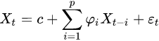
Serial correlation or autocorrelation means that there is persistence in the data; that is, future data can be predicted (to some degree) from past data. Such a quality could indicate the existence of trends.序列相关或自相关意味着数据存在持久性; 也就是说,可以根据过去的数据(在某种程度上)预测未来的数据。 这种质量可能表明趋势的存在。 A simple way of finding autocorrelation is to put the data into column A of a spreadsheet, then copy it to column B while shifting the data down by 1 row. Then find the correlation of column A and column B. Additional correlations can be calculated shifting column B down 2, 3, or 4 rows, which might show the existence of a cycle.
 ), then we may wish to only measure the association between
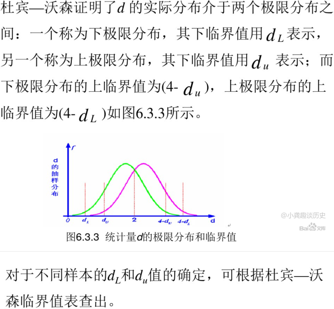
 The Durbin Watson (DW) statistic is a test for autocorrelation in the residuals from a statistical model or regression analysis.(The Durbin Watson statistic is a test for autocorrelation in a regression model's output.) The Durbin-Watson statistic will always have a value ranging between 0 and 4.
A stock price displaying positive autocorrelation would indicate that the price yesterday has a positive correlation on the price today—so if the stock fell yesterday, it is also likely that it falls today. A security that has a negative autocorrelation, on the other hand, has a negative influence on itself over time—so that if it fell yesterday, there is a greater likelihood it will rise today.
A similar assessment can be also carried out with the Breusch–Godfrey test and the Ljung–Box test(ts10_Univariate TS模型_circle mark pAcf_ETS_unpack product_darts_bokeh band interval_ljungbox_AIC_BIC_LIQING LIN的博客-CSDN博客).
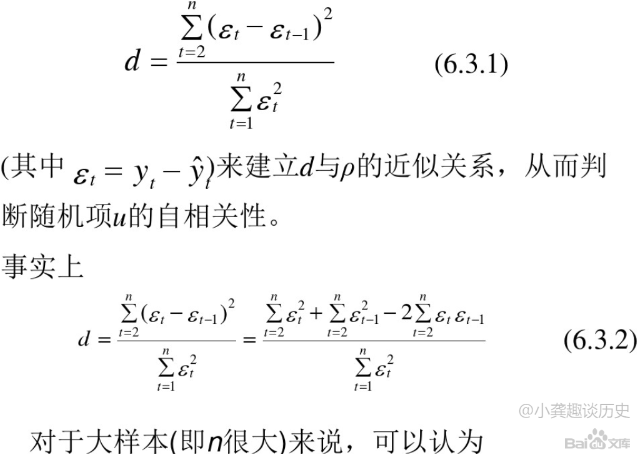
A formal way of finding autocorrelation is by using the Durbin-Watson test, which gives the d-statistic. This approach measures the change in the errors (e), the difference between N data points and their average value.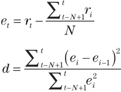
The Hypotheses for the Durbin Watson test are:
(For a first order correlation, the lag is one time unit).
Assumptions are:

 https://www.le.ac.uk/users/dsgp1/COURSES/LEISTATS/Lecture8.pdf
 ts9_annot_arrow_hvplot PyViz interacti_bokeh_STL_seasonal_decomp_HodrickP_KPSS_F-stati_Box-Cox_Ljung_"crosshairtool(dimensions=\"height\")"_LIQING LIN的博客-CSDN博客
Autocorrelation of residuals is a measure of the correlation between the error terms (residuals) of a time series model at different lags. It is important to interpret the autocorrelation of residuals because it can indicate whether the model is adequately capturing all the systematic patterns in the data.
If the autocorrelation of residuals is close to zero for all lags, it suggests that the model is capturing all the systematic patterns in the data, and the residuals are behaving randomly and independently. This is desirable because it indicates that the model is a good fit to the data.
On the other hand, if the autocorrelation of residuals is high for one or more lags, it suggests that the model is not capturing all the systematic patterns in the data. Specifically, it suggests that there is some pattern or trend in the residuals that is not accounted for by the model, and this can lead to biased parameter estimates, inflated standard errors, and invalid test statistics.
If is the residual(the difference between the calculated/observed value and the predicted value for a particular observation) given by
![]() ,
,
############
<== 残差自相关
<==residual measures the relationship between
and
![]() ,
,
==>
![]()
residual measures the relationship between
![]() and
and ,
<==AR(1) = AR(P=1) =![]() In this regression model, the response variable in the previous time period
In this regression model, the response variable in the previous time period ![]() has become the predictor and the errors have our usual assumptions about errors
has become the predictor and the errors have our usual assumptions about errors (white noise) in a simple linear regression model(note
![]() is a constant) https://blog.csdn.net/Linli522362242/article/details/127558757<==
is a constant) https://blog.csdn.net/Linli522362242/article/details/127558757<==
############
the Durbin-Watson test statistic is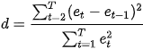
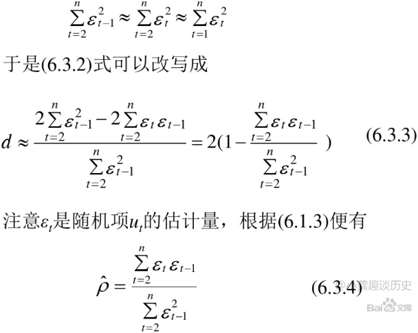
where T is the number of observations. For large T, d is approximately equal to 2(1 − ![]() ), where
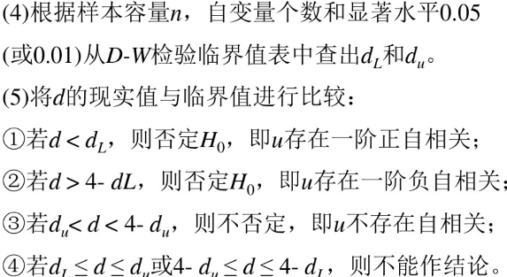
), where ![]() is the sample autocorrelation of the residuals, d = 2 therefore indicates no autocorrelation. The value of d always lies between 0 and 4. If the Durbin–Watson statistic is substantially less than 2(d<2), there is evidence of positive serial correlation. As a rough rule of thumb, if Durbin–Watson is less than 1.0, there may be cause for alarm. Small values of d indicate successive error terms are positively correlated较小的 d 值表示连续误差项呈正相关. If d > 2, successive error terms are negatively correlated. In regressions, this can imply an underestimation of the level of statistical significance.在回归中,这可能意味着低估了统计显着性水平
is the sample autocorrelation of the residuals, d = 2 therefore indicates no autocorrelation. The value of d always lies between 0 and 4. If the Durbin–Watson statistic is substantially less than 2(d<2), there is evidence of positive serial correlation. As a rough rule of thumb, if Durbin–Watson is less than 1.0, there may be cause for alarm. Small values of d indicate successive error terms are positively correlated较小的 d 值表示连续误差项呈正相关. If d > 2, successive error terms are negatively correlated. In regressions, this can imply an underestimation of the level of statistical significance.在回归中,这可能意味着低估了统计显着性水平
A positive autocorrelation, or serial correlation, means that a positive error factor has a good chance of following another positive error factor正自相关或序列相关意味着正误差因子很有可能跟随 另一个正误差因子.https://en.wikipedia.org/wiki/Durbin%E2%80%93Watson_statistic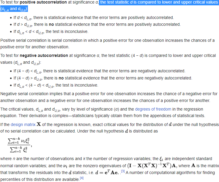
#######(5)6.3自相关的检验 - 百度文库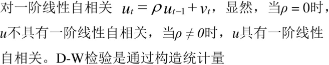


####### https://www.investopedia.com/terms/d/durbin-watson-statistic.asp#:~:text=The%20Durbin%20Watson%20statistic%20is,above%202.0%20indicates%20negative%20autocorrelation.
Assume the following (x,y) data points:
Using the methods of a least squares regression to find the "line of best fit," the equation for the best fit line of this data is:
Y=−2.6268*x +1,129.2
This first step in calculating the Durbin Watson statistic is to calculate the expected "y" values using the line of best fit equation. For this data set, the expected "y" values are:
Next, the differences of the actual "y" values versus the ExpectedY values, the errors, are calculated:
Next these errors must be squared and summed![]() :
:
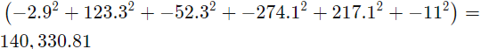
Next, the value of the error minus the previous error are calculated and squared![]() :
:
Finally, the Durbin Watson statistic is the quotient of the squared values:
Durbin Watson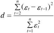 : d=389,406.71/140,330.81=2.77
Note: Tenths place may be off due to rounding errors in the squaringDurbin Watson Test - GeeksforGeeks
FIGURE 2.6 Normal distribution showing the percentage area included within one standard deviation about the arithmetic mean.
If we see the normal distribution (Figure 2.6) as the annual returns for the stock market over the past 50 years, then the mean is about 8%, and one standard deviation is 16%. In any one year, we can expect the returns to be 8%; however, there is a 32% chance that it will be either greater than 24% (= 8% + 16%) or less than –8% (= 8% - 16%). If you would like to know the probability of a return of 20% or greater, you must first rescale the values如果您想知道 20% 或更高回报的概率,您必须首先重新调整值,
If your objective is 20%, we calculate ![]()
Table A1.1, Appendix 1 gives the probability for normal curves. Looking up the standard deviation of 0.75 gives 27.34%, a grouping of 54.68%(=27.34%*2) of the data. That leaves one half of the remaining data, or 22.66%(0.2266=0.5-0.2734 or 0.2266=1-0.7734)), above the target of 20%.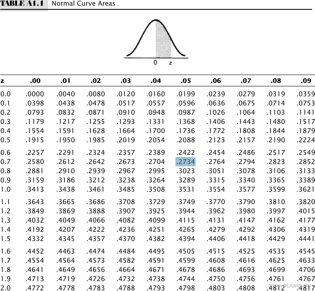
Table A1.1, Appendix 1
使用Table Va的值需要减去0.5
left tail area = right tail area #1_Statistics_agent_policy_explanatory_predictor_response_numeric_mode_Hypothesis_Type I_Chi-squ_LIQING LIN的博客-CSDN博客

# confidence (interval)= 0.95 ==>(1-confidence)/2 = 0.025 (right tail area) ==>1-0.025=0.975
# P(z<Z?) = 0.975 ==> Z=1.96
cdf : P(z<1.96) ==> 0.975 (probability(area) under the curve): calculate the area under the curve that corresponds to a particular z value (the standard deviation)
mpf3_Nonlinearit_Black-Scholes_option_Implied volati_Type I & II_Incremental_bisection_Newton_secant_the volatility is below intrinsic value_LIQING LIN的博客-CSDN博客#left z <== ppf(q, loc=0, scale=1) = ppf(prob, theta, sigma) # Pr(Z<=z) = prob
#right z <== ppf(q, loc=0, scale=1) = ppf(1-prob, theta, sigma) # Pr(Z>=z) = 1-prob mpf5_定价Bond_yield curve_Spot coupon_duration_有效利率_连续复利_远期_Vasicek短期_CIR模型Derivatives_Tridiagonal_ppf_LIQING LIN的博客-CSDN博客
from scipy import stats

xbar=67
mu0=52
s=16.3

# Calculating z-score
z = (xbar-mu0)/s # z = (67-52)/16.3

# Calculating probability under the curve
p_val = 1 - stats.norm.cdf(z)
print( "Prob. to score more than 67 is", round(p_val*100, 2), "%" ) 
It is inconvenient to look up the probability values in a table when you are working with a spreadsheet or computer program, yet the probabilities are easier to understand than standard deviation values. You can calculate the area under the curve that corresponds to a particular z value (the standard deviation), using the following approximation.
Let z′ = |z|, the absolute value of z. Then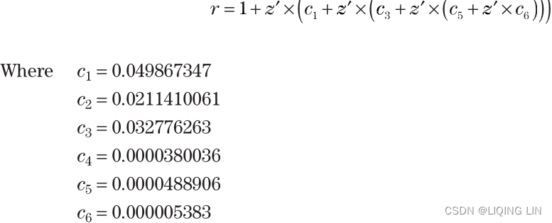
Then the probability, P, that the returns will equal or exceed(>=) the expected return is![]()
Using the example where the standard deviation z = 0.75, we perform the calculation
Substituting the value of into the equation for P, we get![]()
Then there is a 22.7% probability that a value will exceed 0.75 standard deviations (that is, fall on one end of the distribution outside the value of 0.75). The chance of a value falling inside the band formed by ±0.75 standard deviations is 1 – (2 × 0.2266) = 0.5468, or 54.68%. That is the same value found in Table A1.1, Appendix 1.
For those using Excel, the answer can be found with the function normdist(p,mean, stdev,cumulative), where
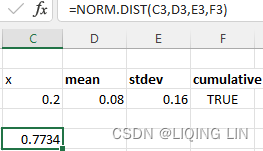 vs
vs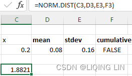
Throughout the development and testing of a trading system, we want to know if the results we are seeing are as expected. The answer will always depend on the size of the data sample and the amount of variance that is typical of the data during this period.
标准误差 (SE) 实际上是统计数据变异性或离散性的度量,例如根据数据样本估计的样本均值。 它被定义为统计量抽样分布的标准差,即从 相同大小和总体的样本中 可以获得的统计量 的所有可能值的分布。
SE 通常用于量化基于样本统计量的 总体参数估计的精度或准确度。 具体来说,假设采样过程重复多次,它提供了样本统计量与真实总体参数之间的平均距离的估计。
SE 使用以下公式计算:
SE = s / sqrt(n),
其中 s 是样本标准差,n 是样本大小。
SE 常用于假设检验和置信区间估计。 在假设检验中(known:sample standard deviation ![]() ),SE 用于计算检验统计量并确定 p 值
),SE 用于计算检验统计量并确定 p 值
###
p_val = stats.t.sf( np.abs(t_sample), n-1 )
print( "Lower tail p-value from t-table: ", p_val )
###
,p 值(P-value)是在 假设原假设为真的情况下 观察到的样本统计量(Critical t value(临界 t 值, ![]() , n-1) from t tables
, n-1) from t tables ![]() )与 根据样本计算出的统计量
)与 根据样本计算出的统计量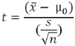 一样极端的概率。 在置信区间估计中,SE 用于围绕样本统计量构建一个区间,该区间可能包含具有一定置信度的真实总体参数。
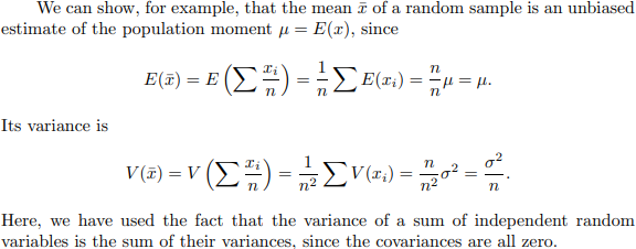
One descriptive measure of error, called the standard error(SE), uses the variance, which gives the estimation of error based on the distribution of the data using multiple data samples. It is a test that determines how the sample means differ from the actual mean of all the data. It addresses解决 the uniformity of the data.
(standard error) SE
Sample means refers to the data being sampled a number of times, each with n data points, and the means of these samples are used to find the variance. In most cases, we would use a single data series and calculate the variance as shown earlier in this chapter.
Unknown:population variance or polulation standard deviation![]()
but, known:sample standard deviation s OR  (9.2)
(9.2)


from scipy import stats
import numpy as np
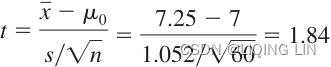
xbar = 7.25 # sample' mean
mu0 = 7 # population's mean
s=1.052 # sample standard deviation
n=60 # sample size
t_sample = (xbar - mu0) / ( s/np.sqrt(float(n)) )
print("Test Statistic t: ", round(t_sample,2))
alpha = 0.05
t_alpha = stats.t.ppf(alpha, n-1) ######right tail
print( "Critical value from t-table: ", -round(t_alpha, 3) )
# upper tail p-value from t-table:
p_val = stats.t.sf( np.abs(t_sample), n-1 )
print( "Upper tail p-value from t-table: ", round(p_val,4) )

TABLE 9.3 Summary of Hypothesis about a Population Mean: ![]() unknown case
unknown case 
When fewer prices or trades are used in a distribution, we can expect the shape of the curve to be more variable. For example, it may be spread out分散 so that the peak of the distribution will be lower分布的峰值较低 and the tails will be higher尾部较高. A way of measuring how close the sample distribution of a smaller set is to the normal distribution (of a large sample of data) is to use the t-statistic测量较小集合的样本分布 与(大数据样本)正态分布 的接近程度的一种方法是使用 t 统计量 (also called the student’s t-test, developed by W. S. Gossett). The t-test is calculated according to its degrees of freedom (df), which is n-1, where n is the sample size, the number of prices used in the distribution.
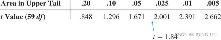
The more data in the sample, the more reliable the results. We can get a broad view of the shape of the distribution by looking at a few values of t in Table 2.2, which gives the values of t corresponding to the upper tail areas of 0.10, 0.05, 0.025, 0.01, and 0.005. The table shows that as the sample size n increases, the values of t approach those of the standard normal values of the tail areas.
The values of t that are needed to be significant can be found in Appendix 1, Table A1.2, “t-Distribution.” The column headed “0.10” gives the 90% confidence level, “0.05” is 95%, and “0.005” is 99.5%. For example, if we had 20 prices in our sample, and wanted the probability of the upper tail to be 0.025, then the value of t would need to be 2.086. For smaller samples, the value of t would be larger in order to have the same confidence.
When testing a trading system, degrees of freedom can be the number of trades produced by the strategy. When you have few trades, the results may not represent what you will get using a longer trading history. When testing a strategy, you will find a similar relationship between the number of trades and the number of parameters, or variables, used in the strategy. The more variables used, the more trades are needed to create expectations with an acceptable confidence level.
You may want to compare two periods of data to decide whether the price patterns have changed significantly. Some analysts use this to eliminate inconsistent data, but the characteristics of price and economic data change as part of the evolving process, and systematic trading should be able to adapt to these changes. This test is best applied to trading results in order to decide if a strategy is performing consistently. This is done with a 2-sample t-test: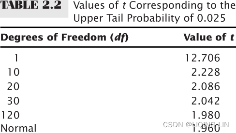
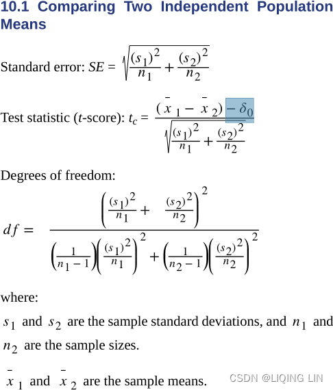 and
and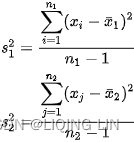
![]()

and the two periods being compared are mutually exclusive. The degrees of freedom, df needed to find the confidence levels in Table A1.2 can be calculated using Satterthwaite’s approximation, where s is the standard deviation of the data values:
When using the t-test to find the consistency of profits and losses generated by a trading system, replace the data items by the net returns of each trade, the number of data items by the number of trades, and calculate all other values using returns rather than prices.
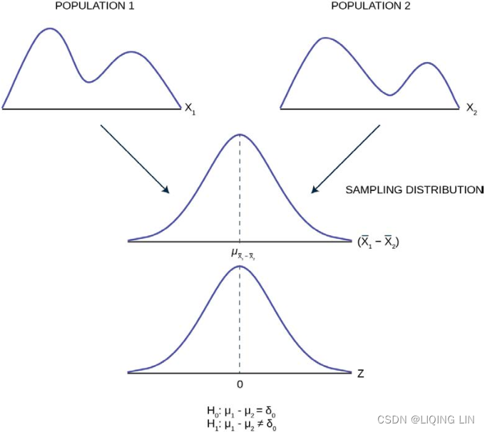
Pictured are
一个有趣的研究问题是不同类型的教学形式对学生成绩的影响(如果有的话)。 为了调查这个问题,我们从混合班级中抽取了一个学生成绩样本,并从标准讲座形式的班级中抽取了另一个样本。 两堂课都是针对同一主题的。 35 名混合学生的平均课程成绩百分比为 74,标准差为 16。标准讲座班的 40 名学生的平均成绩为 76%,标准差为 9。以 5% 进行测试,看看是否存在 标准讲座课程和混合课程之间的总体平均成绩是否存在显着差异。
首先我们注意到我们有两组,来自混合班级的学生和来自标准讲座格式班级的学生。 我们还注意到,我们感兴趣的随机变量是学生的成绩,一个连续随机变量。 我们可以用不同的方式提出研究问题并有一个二元随机变量。 例如,我们可以研究成绩不及格或成绩为 A 的学生的百分比。 这两者都是二元的,因此是比例测试,而不是像这里的情况那样的手段测试。 最后,没有假设哪种格式可能会导致更高的分数,因此假设被表述为双尾检验。
As would virtually always be the case, we do not know the population variances of the two distributions and thus our test statistic is:
To determine the critical value of the Student's t we need the degrees of freedom. For this case we use: df = n1+ n2 - 2 = 35 + 40 -2 = 73. This is large enough to consider it the normal distribution thus = 1.96 <|-0.65|.(落在拒绝域中) Again as always we determine if the calculated value is in the tail determined by the critical value. In this case we do not even need to look up the critical value: the calculated value of the difference in these two average grades is not even one standard deviation apart. Certainly not in the tail.
Conclusion: Cannot reject the null at α=5%. Therefore, evidence does not exist to prove that the grades in hybrid and standard classes differ.
How to Calculate Degrees of Freedom for Any T-Test - Statology
The Welch two-sample t test uses the Satterthwaite DF, which is often smaller than the DF= n1+n2−2 of the pooled 2-sample t test (never larger). This means that the power of the Welch 2-sample t test is somewhat smaller than the power of the pooled test, often not enough smaller to matter for practical purposes. But some statisticians do make an exception to standard practice when sample sizes are very small and sample standard deviations are similar.
In order to compare one trading method with another, it is necessary to standardize both the tests and the measurements used for evaluation. If one system has total returns of 50% and the other 250%, we cannot decide which is best unless we know the duration of the test and the volatility of the returns, or risk.
The return relative to the risk is crucial to performance as will be discussed in Chapter 21, System Testing. For now it is only important that returns and risk be annualized or standardized to make comparisons valid.
The calculations for both 1-period returns and annualized returns will be an essential part of all performance evaluations. In its simplest form, the 1-period rate of return, R, or the holding period rate of return is often given as
For the stock market, which has continuous prices, this can be written
pct_change() command that gives us the percentage change over the prior period values
where is the initial price and
is the price after one period has elapsed. The securities industry often prefers a different calculation,

Note: the logarithmic base to use. Default is 'e' ==> pfc1_whylog return Nominal Inflation_CPI_Realized Volati_outlier_distplot_Jarque–Bera_pAcf_sARIMAx_LIQING LIN的博客-CSDN博客
https://faculty.washington.edu/ezivot/econ424/returnCalculations.pdf
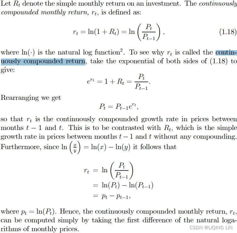
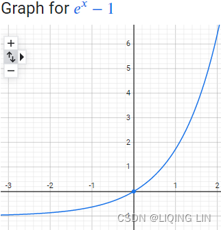

Both methods have advantages and disadvantages. Neither one is the “correct” calculation. Note that in some software, the function log is actually the natural log, and is the log base 10. It is best to always check the definitions. In order to distinguish the two calculations, the first method will be called the standard method and the second the ln method.
In the following spreadsheet example, shown in Table 2.3 over 22 days, the standard returns are in column D and the ln returns in column E. The differences seem small, but the averages are 0.00350 and 0.00339. The standard returns are better by 3.3% over only one trading month. At this rate, the standard method would have yielded returns that were nearly 40%=3.3%*12 higher after one year. The Net Asset Value (NAV), used extensively throughout this book, compounds the periodic returns对定期回报进行复利, and most often has a starting value,.
for NAV using LN
OR and
![]()
Note:
TABLE 2.3 Calculation of Returns and NAVs from Daily Profits and LossesMagic of Log Returns: Practical – Part 2
################https://blog.csdn.net/Linli522362242/article/details/125863306
Compound interest is interest calculated on the initial principal and also on the accumulated interest of previous periods of a deposit or loan. The effect of compound interest depends on frequency.
Assume an annual interest rate of 12%. If we start the year with $100 and compound only once, at the end of the year, the principal grows to $112 (P∗(1+r∗t)=100∗(1+0.12∗1)= $112). Interest applied only to the principal is referred to as simple interest.
If we instead compound each month at 1%(monthly-compounded yield=R=![]() ), we end up with more than $112 at the end of the year(T=1 year). That is,
), we end up with more than $112 at the end of the year(T=1 year). That is,![]() =112.68. (It's higher because we compounded more frequently.)
=112.68. (It's higher because we compounded more frequently.)
If we known the monthly-compounded yield is 1%, and the value is $112.68 after one year, we want to calculate the present value: ![]()
################
In most cases, it is best to standardize the returns by annualizing. This is particularly helpful when comparing two sets of test results, where each covers a different time period. When annualizing, it is important to know that
#########rolling window https://blog.csdn.net/Linli522362242/article/details/122955700
There are exactly 252 trading days in 2021. January and February have the fewest (19), and March the most (23), with an average of 21 per month, or 63 per quarter.
Out of a possible 365 days, 104 days(365/7=52*2=104) are weekend days (Saturday and Sunday) when the stock exchanges are closed. Seven of the nine holidays which close the exchanges fall on weekdays, with Independence Day being observed on Monday, July 5, and Christmas on Friday, December 24. There is one shortened trading session on Friday, November 26 (the day after Thanksgiving Day). ==> 365-104-7-2=252
https://en.wikipedia.org/wiki/Trading_day#:~:text=(Christmas%20Eve).-,2021,the%20stock%20exchanges%20are%20closed.
########
The following formulas use 252 days, which will be the standard throughout this book except for certain interest rate calculations; however, 365 or 360 may be substituted, or even 260 for trading days in other parts of the world.
The Annualized Rate Of Return (AROR) on a simple-interest basis单利 年化回报率 for an investment over n days is 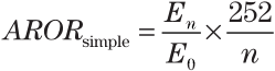
where is the starting equity or account balance,
is the equity at the end of the nth
period, and 252./n are the years expressed as a decimal.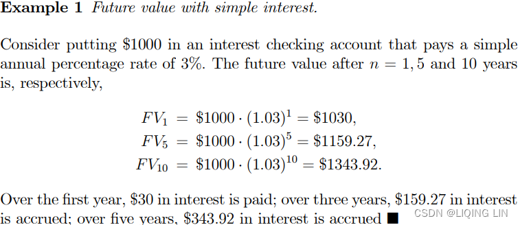
When the 1-period returns are calculated using the standard method, then the annualized compounded rate of return is


Note that AROR or R (capital) refers to the annualized rate of return while is the daily r or 1-period return. Also, the form of the results is different for the two calculations. An increase of 25% for the simple return will show as 0.25 while the same increase using the compounded returns will be 1.25.
When the 1-period returns use the LN method, then the annualized rate of return is the sum of the returns divided by the number of years
and
Annualized Daily Log Return Rate =
![]()
##############
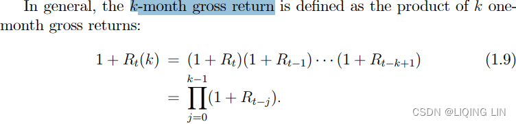
note :
Note: log(ab) = log(a) + log(b)
==>n is the number of years and get the average:
An example of this can be found in column F, the row labeled AROR, in the previous spreadsheet. Note that the annualized returns using the ln method are much lower than those using division and compounding. The compounded method will be used throughout this book.
##############
The use of the standard deviation and compounded rate of return are combined to find the probability of a return objective. In the following calculation, the arithmetic mean of continuous returns is , and it is assumed that the returns are normally distributed.
where
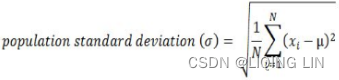
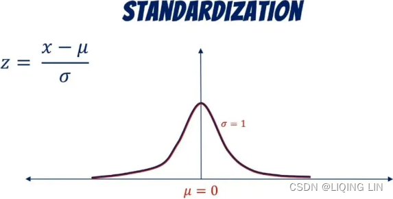
![]() or
or![]()
==> calculate the average:
While we would always like to think about returns, it is even more important to be able to assess risk. With that in mind, there are two extreme risks. The first is event risk, which takes the form of an unpredictable price shock. The worst of these is/ˌkætəˈstrɑːfɪk/灾难性的;极糟的 catastrophic risk, which will cause fatal losses or ruin/ ˈruːɪn /毁灭;破产. The second risk is self-induced自感应的,自诱导的 by overleverage, or gearing up使换快档,增加 your portfolio, until a sequence of bad trades causes ruin. The risk of price shocks and leverage will both be discussed in detail later in other chapters.
The standard risk measurement is useful for comparing the performance of two systems. It is commonly applied to the returns of a single stock or an entire portfolio compared to a benchmark, such as the returns of the S&P 500 or a bond fund. The most common estimate of risk is the standard deviation, σ, of returns, r, shown earlier in this chapter. For most discussions of risk, the standard deviation will also be called volatility. When we refer to the target volatility of a portfolio, we mean the percentage of risk represented by 1 standard deviation of the returns, annualized当我们提到投资组合的目标波动率时,我们指的是年化回报率的 1 个标准差所代表的风险百分比. For example, in the previous spreadsheet, columns D and E show the daily returns. The standard deviations of those returns are shown in the same columns in the row “Std Dev” as 0.01512 and 0.01495. Looking only at column D, 1 standard deviation of 0.01502 means that there is a 68.26% chance of a daily profit or loss less than 1.502%. However, target volatility always refers to annualized risk, and to change a daily return to an annualized one we simply multiply by ![]() . Then the daily standard deviation of returns of 1.512% becomes an annualized volatility of 23.8%, also shown at the bottom of the spreadsheet example. Because we only care about the downside risk, there is a 15.86% chance that we could lose greater than 23.84% in one year. The greater the standard deviation of returns, the greater the risk.
. Then the daily standard deviation of returns of 1.512% becomes an annualized volatility of 23.8%, also shown at the bottom of the spreadsheet example. Because we only care about the downside risk, there is a 15.86% chance that we could lose greater than 23.84% in one year. The greater the standard deviation of returns, the greater the risk.
import scipy.stats as stats

mu = 0.00350    # np.mean( daily_returns )
sigma = 0.01502 # np.std( daily_returns )

stats.norm.cdf(mu+sigma, mu, sigma) - stats.norm.cdf(mu-sigma, mu, sigma)![]() #68.26% chance of a daily profit or loss less than 1.502%
#68.26% chance of a daily profit or loss less than 1.502%
Annualized Average Return = (1 + Daily Average Return) ^ 252 - 1
= (1 + 0.00350) ^ 252 - 1
= 1.4120091974741036 (expressed as a negative value, since the average return is less than 1)
Annualized Volatility = Daily Standard Deviation * sqrt(252) * 100%
= 0.01502 * sqrt(252) * 100%
= 0.2384 or 23.84%
annual_mean = mu/252
annual_std = sigma*np.sqrt(252)#0.2384 # target volatility

stats.norm.cdf(annual_mean-annual_std, annual_mean, annual_std) ![]() # the probabiliy of the loss <= annual_mean-annual_std # left tail area
# the probabiliy of the loss <= annual_mean-annual_std # left tail area
Beta (β) is commonly used in the securities industry to express the relationship of a single market to an portfolio or index. If beta is zero then there is no relationship; if it is positive then the single series tends to move with the index, both above and below. As beta gets larger the volatility of the single market tends to be increasingly greater than the index. Specifically,
A negative beta is similar to a negative correlation, where the moves of the market are generally opposite to the index.
Beta is found by calculating the linear regression of the single market with the index. It is the slope of the single market divided by the slope of the index. Alpha, the added value, is the y-intercept of the solution. The values can be found using Excel, and are discussed in detail in Chapter 6. A general formula for beta is![]()
where A is the single market and B is a portfolio or index.
annual_std =0.12
stats.norm.cdf(annual_mean-annual_std, annual_mean, annual_std) ![]()
If we have a target volatility of 12%, that is, we are willing to accept a 16% chance of losing 12% in one year, but the actual returns show an annualized volatility of 23.8% based on an investment of $100,000, then to correct to a 12% target we simply increase the investment by 23.8/12.0=1.98, or a factor of 1.98 to $198,000, while holding the same position size(incorrect). This is essentially deleveraging your positions by trading a smaller percentage of your account value(not accurate)去杠杆化通常是指减少投资组合中借入资金或杠杆的数量,而本声明是指调整投资规模以达到所需的波动水平. Alternatively, we can reduce the position size by dividing by 1.98 and keeping the investment the same(也无法达到预期目标。 这只会减少标的资产的风险敞口exposure, 并按比例减少潜在收益和损失).
All results in this book will be shown at the target volatility of 12% unless otherwise stated. This is considered a modest risk level, which can be as high as 18% for some hedge funds. It will allow you to compare various systems and test results and see them at a level of risk that is most likely to represent targeted trading results.
The previous examples used daily data and an annualization factor of ![]() . For monthly data, which is most common in published performance tables, we would take the monthly returns and multiply by 12
. For monthly data, which is most common in published performance tables, we would take the monthly returns and multiply by 12![]() . In general, annualizing can be done by multiplying the data by the square root of the number of data items in a year. Then we use 252 for daily data, 12 for monthly, 4 for quarterly, and so on.
. In general, annualizing can be done by multiplying the data by the square root of the number of data items in a year. Then we use 252 for daily data, 12 for monthly, 4 for quarterly, and so on.
The daily expected return formula is:
Expected Daily Return = (Sum of Daily Returns) / (Number of Observations)
For example, if a stock has daily returns of 0.2%, -0.1%, 0.3%, -0.4%, and 0.1% over a five-day period, the expected daily return would be:
(0.2% - 0.1% + 0.3% - 0.4% + 0.1%) / 5 = 0.02%
For example, if a stock has a daily return of 0.2%, the annualized daily return would be:
Annualized Daily Return = (1 + 0.2%) ^ 252 - 1 = 64.14%
This means that if the stock continues to perform at the same rate as it did over the past year, the annualized return would be approximately 64.14%.
The daily expected return gives you an idea of the average return you can expect to earn on a daily basis, while the annualized daily return gives you an idea of the average return you can expect to earn over a one-year period, after compounding the returns.
Although monthly performance results are common in financial disclosure documents, this convention works to the advantage of the person publishing the performance. It is unlikely that the highest or lowest daily net asset value (NAV) will occur on the last day of the month, so the extremes will rarely be seen, and the performance statistics will appear smoother than when using daily returns. Those responsible for due diligence before investing in a new product will often require daily return data in order to avoid overlooking a large drawdown that occurred mid-month.
Using the S&P index as an example, the annualized volatility of the daily returns from 1990 through 2010 was 18.6%, but based on monthly returns it was only 15.3%. The risk based on monthly returns is 17.7% lower, but the annualized rate of return would be the same because it only uses the beginning and ending values.
Because the standard deviation is symmetric, a series of jumps in profits will be interpreted as larger risk. Some analysts believe that it is more accurate to measure the risk as limited to only the downside returns or drawdowns. The use of only losses is called lower partial moments, where lower refers to the downside risk, and partial means where only one side of the return distribution is used. The easiest way to see this is semi-variance, which measures the dispersion that falls below the mean, , or some target value测量低于平均值
或某个目标值的离差,
 OR
OR
Suppose you are analyzing the daily returns of a stock over the last month. The daily returns are as follows:
Day 1: -1%
Day 2: 2%
Day 3: -3%
Day 4: -1%
Day 5: 0%
Day 6: 1%
Day 7: -2%
Day 8: -1%
Day 9: 0%
Day 10: 1%
Day 11: -2%
Day 12: -1%
Day 13: -3%
Day 14: 0%
You want to calculate the semivariance for the returns that are below 0%. To do this, you first need to calculate the average return for the entire period:
Average Daily Return = (Sum of Daily Returns) / (Number of Observations)
= (-1% + 2% - 3% - 1% + 0% + 1% - 2% - 1% + 0% + 1% - 2% - 1% - 3% + 0%) / 14
= -0.357%
daily_return=np.array( [-0.01, 0.02,-0.03,-0.01,
               0.00, 0.01, -0.2, -0.01,
               0.00, 0.01, 0.2, -0.01,
               -0.03, 0.01
              ])
np.mean(daily_return)![]()
Next, you need to calculate the number of observations where the returns are below -0.357% and the squared deviation of those returns from the average return:
def semi_var(ser):
    average = np.nanmean(ser)
    r_below = ser[ser < average]
    return 1/len(r_below) * np.sum( (average - r_below)**2 )
semi_var(daily_return)![]()
However, the most common calculation for system performance is to take the daily drawdowns, that is, the net loss on each day that the total equity is below the peak equity. For example, if the system returns had produced an equity of $25,000 on day t, followed by a daily loss of $500, and another loss of $250, then we would have two values as input 500/25000=0.02 and 750/25000= 0.03. Only those net returns below the most recent peaks are used in the semivariance calculation只有那些低于最近峰值的净回报才会用于半方差计算. Alternatively, you could just take the standard deviation of these daily drawdowns to find the probable size of the drawdowns.或者,您可以仅采用这些每日回撤的标准差来找出可能的回撤规模
One concern about using only the drawdowns to predict other drawdowns is that it limits the number of cases and discards the likelihood that higher-than-normal profits can be related to higher overall risk. In situations where there are limited amounts of test data, using both the gains and losses will give more robust results. When there is a large amount of data, the use of drawdowns can be a very good measurement.
A full discussion of performance measurements can be found in Chapter 21, System Testing, and also in Chapter 23 under the headings “Measuring Return and Risk” and “Ulcer Index.”
The purpose of an average is to transform individuality into classification. In doing that, the data is often smoothed, and useful information is gained. Indexes have attracted enormous popularity in recent years. Where there was only the Value Line and S&P 500 trading as futures markets in the early 1980s, now there are stock index futures contracts representing the markets of every industrialized country. The creation of trusts, such as SPDRs (called “Spyders,” the S&P 500, ^GSPC), Diamonds (DIA, the Dow Jones Industrials, ^DJI), and Qs (QQQ, the NASDAQ 100, ^IXIC) have given stock traders a familiar vehicle to invest in the broad market rather than pick individual shares. Industrial sectors, such as pharmaceuticals/ˌfɑ:məˈsju:tɪkəlz/制药, health care, and technology, first appeared as mutual funds, then as ETFs, and now can also be traded as futures. These index markets all have the additional advantage of not being constrained by having to borrow shares in order to sell short, or by the uptick rule (if it is reinstated) requiring all short sales to be initiated on an uptick in price这些指数市场都具有额外的优势,即不受必须借入股票才能卖空的限制,也不受要求所有卖空都在价格上涨时启动的上涨规则(如果恢复)的限制.
Index markets allow both individual and institutional participants a number of specialized investment strategies. They can buy or sell the broad market, they can switch from one sector to another (sector rotation板块轮换), or they can sell an overpriced sector while buying the broad market index (statistical arbitrage). Institutions find it very desirable, from the view of both costs and taxes, to temporarily hedge their cash stock portfolio by selling S&P 500 futures rather than liquidating stock positions. They may also hedge using options on the S&P futures or SPYs. An index simplifies the decision-making process for trading. If an index does not exist, one can be constructed to satisfy most purposes.
The index holds an important role as a benchmark for performance. Most investors believe that a trading program is only attractive if it has a better return-to-risk ratio than a portfolio of 60% stocks (as represented by the S&P 500 index), and 40% bonds (the Lehman Brothers Treasury Index). Beating the index is called creating alpha, proving that you’re smarter than the market.
An index is standardized way of expressing price movement, normally an accumulation of percentage changes. Most indexes have a starting value of 100 on a specific date. The selection of the base year is often “convenient” but can be chosen as a period of price stability. The base year for U.S. productivity and for unemployment is 1982; for consumer confidence, 1985; and for the composite of leading indicators, 1987. The CRB Yearbook shows the Producer Price Index (PPI) from as far back as 1913. For example, the PPI, which is released monthly, had a value of 186.8 in October 2010 and 185.1 in September 2010, a 0.9184%=(186.8/185.1-1)x100% increase in one month. An index value less than 100 means that the index has less value than when it started.
Each index value is calculated from the previous value as:![]()
and the 1-period returns are calculated in the same way as shown previously in this chapter.
The last calculations shown in the spreadsheet, Table 2.3, are the Net Asset Value (NAV), calculated two ways. This is essentially the returns converted to an index, showing the compounded rate of return based on daily profit and losses relative to a starting investment. In the spreadsheet, this is shown in column F using standard returns and G using LN returns.
The process of calculating NAVs can be done with the following steps:
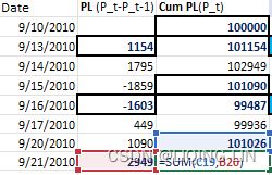

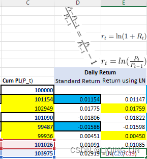
 and if using method (b) then each

The final values of the NAV are in the last dated rows. The U.S. government requires that NAVs be calculated this way, although it doesn’t specify whether returns should be based on the natural log. This process is also identical to indexing, which turns any price series into one that reflects percentage returns.