基于距离正则的水平集分割MATLAB代码,无需初始化
%  This Matlab code demonstrates an edge-based active contour model as an application of
%  the Distance Regularized Level Set Evolution (DRLSE) formulation in the following paper:
%
%  C. Li, C. Xu, C. Gui, M. D. Fox, "Distance Regularized Level Set Evolution and Its Application to Image Segmentation",
%     IEEE Trans. Image Processing, vol. 19 (12), pp. 3243-3254, 2010.
%
% Author: Chunming Li, all rights reserved
% E-mail: lchunming@gmail.com
%         li_chunming@hotmail.com
% URL:  http://www.imagecomputing.org/~cmli//
clear all;
close all;
Img=imread('gourd.bmp');
Img=double(Img(:,:,1));
%% parameter setting
timestep=1;  % time step
mu=0.2/timestep;  % coefficient of the distance regularization term R(phi)
iter_inner=5;
iter_outer=20;
lambda=5; % coefficient of the weighted length term L(phi)
alfa=-3;  % coefficient of the weighted area term A(phi)
epsilon=1.5; % papramater that specifies the width of the DiracDelta function
sigma=.8;    % scale parameter in Gaussian kernel
G=fspecial('gaussian',15,sigma); % Caussian kernel
Img_smooth=conv2(Img,G,'same');  % smooth image by Gaussiin convolution
[Ix,Iy]=gradient(Img_smooth);
f=Ix.^2+Iy.^2;
g=1./(1+f);  % edge indicator function.
% initialize LSF as binary step function
c0=2;
initialLSF = c0*ones(size(Img));
% generate the initial region R0 as two rectangles
initialLSF(25:35,20:25)=-c0;
initialLSF(25:35,40:50)=-c0;
phi=initialLSF;
figure(1);
mesh(-phi);   % for a better view, the LSF is displayed upside down
hold on;  contour(phi, [0,0], 'r','LineWidth',2);
title('Initial level set function');
view([-80 35]);
figure(2);
imagesc(Img,[0, 255]); axis off; axis equal; colormap(gray); hold on;  contour(phi, [0,0], 'r');
title('Initial zero level contour');
pause(0.5);
potential=2;
if potential ==1
    potentialFunction = 'single-well';  % use single well potential p1(s)=0.5*(s-1)^2, which is good for region-based model
elseif potential == 2
    potentialFunction = 'double-well';  % use double-well potential in Eq. (16), which is good for both edge and region based models
else
    potentialFunction = 'double-well';  % default choice of potential function
end
% start level set evolution
for n=1:iter_outer
    phi = drlse_edge(phi, g, lambda, mu, alfa, epsilon, timestep, iter_inner, potentialFunction);
    if mod(n,2)==0
        figure(2);
        imagesc(Img,[0, 255]); axis off; axis equal; colormap(gray); hold on;  contour(phi, [0,0], 'r');
    end
end
% refine the zero level contour by further level set evolution with alfa=0
alfa=0;
iter_refine = 10;
phi = drlse_edge(phi, g, lambda, mu, alfa, epsilon, timestep, iter_inner, potentialFunction);
finalLSF=phi;
figure(2);
imagesc(Img,[0, 255]); axis off; axis equal; colormap(gray); hold on;  contour(phi, [0,0], 'r');
hold on;  contour(phi, [0,0], 'r');
str=['Final zero level contour, ', num2str(iter_outer*iter_inner+iter_refine), ' iterations'];
title(str);
figure;
mesh(-finalLSF); % for a better view, the LSF is displayed upside down
hold on;  contour(phi, [0,0], 'r','LineWidth',2);
view([-80 35]);
str=['Final level set function, ', num2str(iter_outer*iter_inner+iter_refine), ' iterations'];
title(str);
axis on;
[nrow, ncol]=size(Img);
axis([1 ncol 1 nrow -5 5]);
set(gca,'ZTick',[-3:1:3]);
set(gca,'FontSize',14)
function phi = drlse_edge(phi_0, g, lambda,mu, alfa, epsilon, timestep, iter, potentialFunction)
%  This Matlab code implements an edge-based active contour model as an
%  application of the Distance Regularized Level Set Evolution (DRLSE) formulation in Li et al's paper:
%
%      C. Li, C. Xu, C. Gui, M. D. Fox, "Distance Regularized Level Set Evolution and Its Application to Image Segmentation",
%        IEEE Trans. Image Processing, vol. 19 (12), pp.3243-3254, 2010.
%
%  Input:
%      phi_0: level set function to be updated by level set evolution
%      g: edge indicator function
%      mu: weight of distance regularization term
%      timestep: time step
%      lambda: weight of the weighted length term
%      alfa:   weight of the weighted area term
%      epsilon: width of Dirac Delta function
%      iter: number of iterations
%      potentialFunction: choice of potential function in distance regularization term.
%              As mentioned in the above paper, two choices are provided: potentialFunction='single-well' or
%              potentialFunction='double-well', which correspond to the potential functions p1 (single-well)
%              and p2 (double-well), respectively.%
%  Output:
%      phi: updated level set function after level set evolution
%
% Author: Chunming Li, all rights reserved
% E-mail: lchunming@gmail.com
%         li_chunming@hotmail.com
% URL:  http://www.imagecomputing.org/~cmli/
phi=phi_0;
[vx, vy]=gradient(g);
for k=1:iter
    phi=NeumannBoundCond(phi);
    [phi_x,phi_y]=gradient(phi);
    s=sqrt(phi_x.^2 + phi_y.^2);
    smallNumber=1e-10;
    Nx=phi_x./(s+smallNumber); % add a small positive number to avoid division by zero
    Ny=phi_y./(s+smallNumber);
    curvature=div(Nx,Ny);
    if strcmp(potentialFunction,'single-well')
        distRegTerm = 4*del2(phi)-curvature;  % compute distance regularization term in equation (13) with the single-well potential p1.
    elseif strcmp(potentialFunction,'double-well');
        distRegTerm=distReg_p2(phi);  % compute the distance regularization term in eqaution (13) with the double-well potential p2.
    else
        disp('Error: Wrong choice of potential function. Please input the string "single-well" or "double-well" in the drlse_edge function.');
    end
    diracPhi=Dirac(phi,epsilon);
    areaTerm=diracPhi.*g; % balloon/pressure force
    edgeTerm=diracPhi.*(vx.*Nx+vy.*Ny) + diracPhi.*g.*curvature;
    phi=phi + timestep*(mu*distRegTerm + lambda*edgeTerm + alfa*areaTerm);
end
function f = distReg_p2(phi)
% compute the distance regularization term with the double-well potential p2 in eqaution (16)
[phi_x,phi_y]=gradient(phi);
s=sqrt(phi_x.^2 + phi_y.^2);
a=(s>=0) & (s<=1);
b=(s>1);
ps=a.*sin(2*pi*s)/(2*pi)+b.*(s-1);  % compute first order derivative of the double-well potential p2 in eqaution (16)
dps=((ps~=0).*ps+(ps==0))./((s~=0).*s+(s==0));  % compute d_p(s)=p'(s)/s in equation (10). As s-->0, we have d_p(s)-->1 according to equation (18)
f = div(dps.*phi_x - phi_x, dps.*phi_y - phi_y) + 4*del2(phi);
function f = div(nx,ny)
[nxx,junk]=gradient(nx);
[junk,nyy]=gradient(ny);
f=nxx+nyy;
function f = Dirac(x, sigma)
f=(1/2/sigma)*(1+cos(pi*x/sigma));
b = (x<=sigma) & (x>=-sigma);
f = f.*b;
function g = NeumannBoundCond(f)
% Make a function satisfy Neumann boundary condition
[nrow,ncol] = size(f);
g = f;
g([1 nrow],[1 ncol]) = g([3 nrow-2],[3 ncol-2]);
g([1 nrow],2:end-1) = g([3 nrow-2],2:end-1);
g(2:end-1,[1 ncol]) = g(2:end-1,[3 ncol-2]);
LeveSet 水平集方法主要的思想是利用三维(高维)曲面的演化来表示二维曲线的演化过程。在计算机视觉领域,利用水平集方法可以实现很好的图像分割效果。
1.数学原理
根据维基百科的定义,在数学上一个包含n个变量的实值函数其水平集可以表示为下面的公式:
L
c
(
f
)
=
(
x
1
,
x
2
,
.
.
.
,
x
n
)
∣
f
(
x
1
,
x
2
,
.
.
.
,
x
n
)
=
c
L
c
(
f
)
=
(
x
1
,
x
2
,
.
.
.
,
x
n
)
∣
f
(
x
1
,
x
2
,
.
.
.
,
x
n
)
=
c
L
c
(
f
)
=
(
x
1
,
x
2
,
.
.
.
,
x
n
)
∣
f
(
x
1
,
x
2
,
.
.
.
,
x
n
)
=
c
Lc(f)=(x1,x2,...,xn)∣f(x1,x2,...,xn)=cL_c(f) = {(x_1,x_2,...,x_n)|f(x_1,x_2,...,x_n) = c}Lc(f)=(x1,x2,...,xn)∣f(x1,x2,...,xn)=c
Lc(f)=(x1,x2,...,xn)∣f(x1,x2,...,xn)=cLc(f)=(x1,x2,...,xn)∣f(x1,x2,...,xn)=cLc(f)=(x1,x2,...,xn)∣f(x1,x2,...,xn)=c
可以看出,水平集指的是这个函数的取值为一个给定的常数c.那么当变量个数为2时,这个函数的水平集就变味了一条曲线,也可以成为等高线。这时函数f就可以描述一个曲面。(同样,三个变量时就能得到一个等值面,大于3的就是水平超面了)
下面来看一个简单的曲面的水平集(等值线的例子):


上图中,左边是Himmelblau方程所描述的曲面即
z
=
f
(
x
,
y
)
z
=
f
(
x
,
y
)
z
=
f
(
x
,
y
)
z=f(x,y)z=f(x,y)z=f(x,y)
z=f(x,y)z=f(x,y)z=f(x,y),右边就是这个曲面的等高线集合,其中每一条就对应着一个常数c的水平集。
2.水平集方法
在计算机视觉中,利用水平集方法的优势在于,可以利用这种方法在固定的坐标系中,计算曲线、曲面的演化,而无需知道曲线曲面的参数,所以这种方法又称为几何法。
具体来讲,在图像分割任务中如果要得到每个物体准确的包络曲线,就需要对去描述这个曲线在xy坐标系下的演化。最初曲线在二维图像平面上是这样的:
y
=
g
(
x
)
y
=
g
(
x
)
y
=
g
(
x
)
y=g(x)y=g(x)y=g(x)
y=g(x)y=g(x)y=g(x)
图割过程就是要找出一条比较好的曲面来包围物体。
但是这个函数求解和计算比较困难,那么就可以用水平集的思想和方法来解决:
1.首先将这个曲线看成是某个三维曲面下的某一条等高线:
z
=
f
(
x
,
y
)
z
=
f
(
x
,
y
)
z
=
f
(
x
,
y
)
z=f(x,y)z = f(x,y)z=f(x,y)
z=f(x,y)z=f(x,y)z=f(x,y)
f
(
x
,
y
)
f
(
x
,
y
)
f
(
x
,
y
)
f(x,y)f(x,y)f(x,y)
f(x,y)f(x,y)f(x,y)就可以看做是一个xy的隐函数方程。
2.特别的,在二维图像领域一般将上面讲到的函数
z
=
f
(
x
,
y
)
z
=
f
(
x
,
y
)
z
=
f
(
x
,
y
)
z=f(x,y)z=f(x,y)z=f(x,y)
z=f(x,y)z=f(x,y)z=f(x,y)设置为0,刚刚所说的曲面的零水平集就是图像上的边缘包络。
z
=
f
(
x
,
y
)
=
0
z
=
f
(
x
,
y
)
=
0
z
=
f
(
x
,
y
)
=
0
z=f(x,y)=0z=f(x,y)=0z=f(x,y)=0
z=f(x,y)=0z=f(x,y)=0z=f(x,y)=0
或者更为标准的形式如下:
Γ
=
(
x
,
y
)
∣
z
(
x
,
y
)
=
0
Γ
=
(
x
,
y
)
∣
z
(
x
,
y
)
=
0
Γ
=
(
x
,
y
)
∣
z
(
x
,
y
)
=
0
Γ=(x,y)∣z(x,y)=0\Gamma = {(x,y)| z(x,y)=0}Γ=(x,y)∣z(x,y)=0
Γ=(x,y)∣z(x,y)=0Γ=(x,y)∣z(x,y)=0Γ=(x,y)∣z(x,y)=0
这时,z(x,y)=f(x,y)就是辅助函数,用三维的曲面来辅助表示二维的曲线。
这里还有一个假设,
Γ
Γ
Γ
Γ\GammaΓ
ΓΓΓ零水平集内部的(包络内的)为正外面为负。
这里有个重要的性质,基于高维曲面水平集方法得到的这个零水平集曲线是封闭的、连续的、处处可导的,这就为后面的图像分割提供了基础。
3.零水平集演化
为了获得与图像边缘相适应的结果,z需要进行演化才能使得其0水平集所描述的曲线很好的包裹住需要分割的物体,那么此时就涉及到方程的演化:
Γ
(
t
)
=
(
x
,
y
)
∣
z
(
x
,
y
)
=
0
Γ
(
t
)
=
(
x
,
y
)
∣
z
(
x
,
y
)
=
0
Γ
(
t
)
=
(
x
,
y
)
∣
z
(
x
,
y
)
=
0
Γ(t)=(x,y)∣z(x,y)=0\Gamma(t) = {(x,y)| z(x,y)=0}Γ(t)=(x,y)∣z(x,y)=0
Γ(t)=(x,y)∣z(x,y)=0Γ(t)=(x,y)∣z(x,y)=0Γ(t)=(x,y)∣z(x,y)=0
∂
z
∂
t
=
v
∣
Δ
z
∣
∂
z
∂
t
=
v
∣
Δ
z
∣
∂
t
∂
z
=
v
∣
Δ
z
∣
∂z∂t=v∣Δz∣\dfrac{\partial z}{\partial t} = v |\Delta z|∂t∂z=v∣Δz∣
∂z∂t=v∣Δz∣∂t∂z=v∣Δz∣∂t∂z=v∣Δz∣
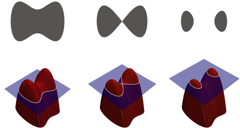
这里是一个曲面演化后,其零水平集演化的过程:
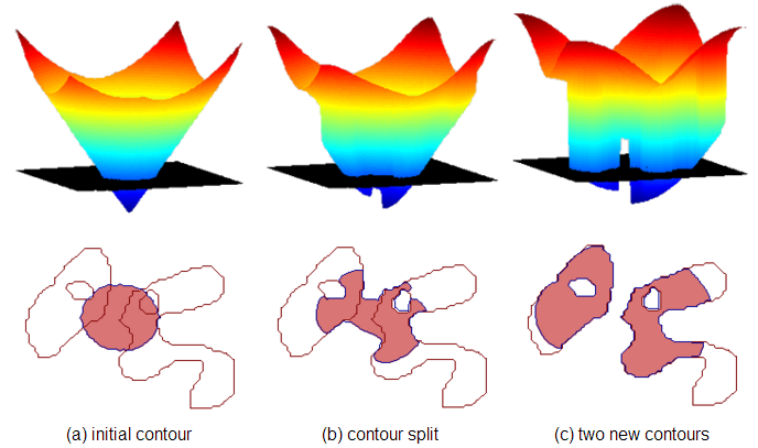
要促使边缘演化成包络object的形式,需要一个所谓的图像力来促使其变化,这时候就需要利用图像中的梯度来作为这个图像力的组成部分驱动曲线去靠近边缘。下图是一个例子,作图是原图,右图是梯度图。
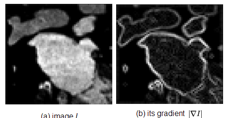
<font color=dodgerblue<那么这个图像力就需要在原理边缘的时候大,靠近边缘的时候缩小,直到贴合边缘。
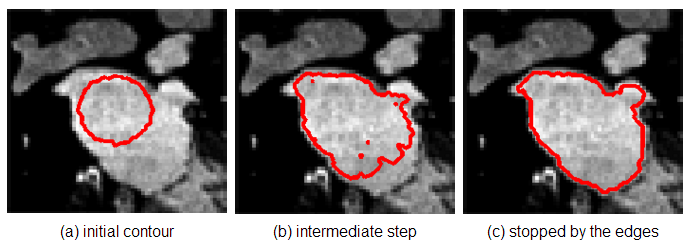
在梯度的驱动下,其演化过程如上图所示。
4.如何求解最小值
上面的问题在数学中可以归结为能量泛函问题,求解边缘的过程就是这个水平集能量泛函最小化的过程。
著名的方法来自于下面这篇文章:
Level Set Evolution Without Re-initialization: A New Variational Formulation
作者(李明纯)通过引入了内部能量项来惩罚由信号距离函数造成的水平集函数的偏差,以及外部能量项来驱动零水平集向期望的图像特征运动,实现了很好的分割效果。
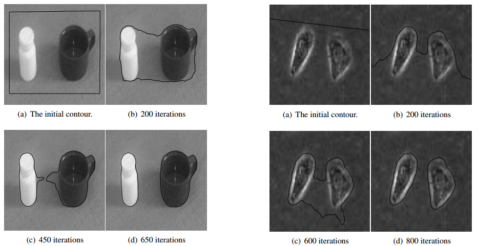
5.Demo
下图是matlab 中,稍作修改运行作者给出的工具函数demo:
原图和分割效果图:

pics contenx ref from:
https://profs.etsmtl.ca/hlombaert/algorithms.php
https://math.berkeley.edu/~sethian/2006/Explanations/level_set_explain.html
https://www.zhihu.com/question/22608763
https://blog.csdn.net/github_35768306/article/details/64129197
https://blog.csdn.net/songzitea/article/details/46385271
李明纯:http://www.engr.uconn.edu/~cmli/
paper:http://www.imagecomputing.org/~cmli/paper/levelset_cvpr05.pdf
matlab:https://www.mathworks.com/matlabcentral/profile/authors/870631-chunming-li
https://blog.csdn.net/yutianxin123/article/details/69802364
cells: https://www.histology.leeds.ac.uk/blood/blood_wbc.php