深度学习中的优化算法之NAG

      之前在https://blog.csdn.net/fengbingchun/article/details/124648766 介绍过Momentum SGD，这里介绍下深度学习的另一种优化算法NAG。

      NAG：Nesterov Accelerated Gradient或Nesterov momentum，是梯度优化算法的扩展，在基于Momentum SGD的基础上作了改动。如下图所示，截图来自：https://arxiv.org/pdf/1609.04747.pdf

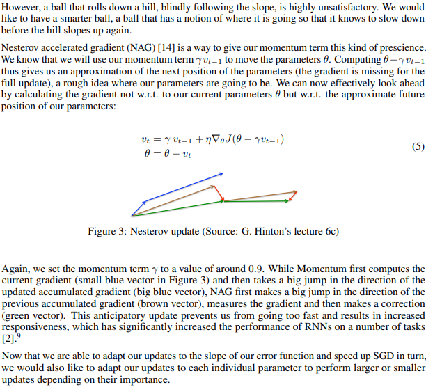
       基于动量的SGD在最小点附近会震荡，为了减少这些震荡，我们可以使用NAG。NAG与基于动量的SGD的区别在于更新梯度的方式不同。

       以下是与Momentum SGD不同的代码片段：

       1. 在原有枚举类Optimization的基础上新增NAG：

enum class Optimization {
	BGD, // Batch Gradient Descent
	SGD, // Stochastic Gradient Descent
	MBGD, // Mini-batch Gradient Descent
	SGD_Momentum, // SGD with Momentum
	AdaGrad, // Adaptive Gradient
	RMSProp, // Root Mean Square Propagation
	Adadelta, // an adaptive learning rate method
	Adam, // Adaptive Moment Estimation
	AdaMax, // a variant of Adam based on the infinity norm
	NAG // Nesterov Accelerated Gradient
};

       2. 计算z的方式不同：NAG使用z2

float LogisticRegression2::calculate_z(const std::vector<float>& feature) const
{
	float z{0.};
	for (int i = 0; i < feature_length_; ++i) {
		z += w_[i] * feature[i];
	}
	z += b_;

	return z;
}

float LogisticRegression2::calculate_z2(const std::vector<float>& feature, const std::vector<float>& vw) const
{
	float z{0.};
	for (int i = 0; i < feature_length_; ++i) {
		z += (w_[i] - mu_ * vw[i]) * feature[i];
	}
	z += b_;

	return z;
}

       3. calculate_gradient_descent函数：

void LogisticRegression2::calculate_gradient_descent(int start, int end)
{
	switch (optim_) {
		case Optimization::NAG: {
			int len = end - start;
			std::vector<float> v(feature_length_, 0.);
			std::vector<float> z(len, 0), dz(len, 0);
			for (int i = start, x = 0; i < end; ++i, ++x) {
				z[x] = calculate_z2(data_->samples[random_shuffle_[i]], v);
				dz[x] = calculate_loss_function_derivative(calculate_activation_function(z[x]), data_->labels[random_shuffle_[i]]);

				for (int j = 0; j < feature_length_; ++j) {
					float dw = data_->samples[random_shuffle_[i]][j] * dz[x];
					v[j] = mu_ * v[j] + alpha_ * dw; // formula 5
					w_[j] = w_[j] - v[j];
				}

				b_ -= (alpha_ * dz[x]);
			}
		}
			break;
		case Optimization::AdaMax: {
			int len = end - start;
			std::vector<float> m(feature_length_, 0.), u(feature_length_, 1e-8), mhat(feature_length_, 0.);
			std::vector<float> z(len, 0.), dz(len, 0.);
			float beta1t = 1.;
			for (int i = start, x = 0; i < end; ++i, ++x) {
				z[x] = calculate_z(data_->samples[random_shuffle_[i]]);
				dz[x] = calculate_loss_function_derivative(calculate_activation_function(z[x]), data_->labels[random_shuffle_[i]]);

				beta1t *= beta1_;

				for (int j = 0; j < feature_length_; ++j) {
					float dw = data_->samples[random_shuffle_[i]][j] * dz[x];
					m[j] = beta1_ * m[j] + (1. - beta1_) * dw; // formula 19
					u[j] = std::max(beta2_ * u[j], std::fabs(dw)); // formula 24

					mhat[j] = m[j] / (1. - beta1t); // formula 20

					// Note: need to ensure than u[j] cannot be 0.
					// (1). u[j] is initialized to 1e-8, or
					// (2). if u[j] is initialized to 0., then u[j] adjusts to (u[j] + 1e-8)
					w_[j] = w_[j] - alpha_ * mhat[j] / u[j]; // formula 25
				}

				b_ -= (alpha_ * dz[x]);
			}
		}
			break;
		case Optimization::Adam: {
			int len = end - start;
			std::vector<float> m(feature_length_, 0.), v(feature_length_, 0.), mhat(feature_length_, 0.), vhat(feature_length_, 0.);
			std::vector<float> z(len, 0.), dz(len, 0.);
			float beta1t = 1., beta2t = 1.;
			for (int i = start, x = 0; i < end; ++i, ++x) {
				z[x] = calculate_z(data_->samples[random_shuffle_[i]]);
				dz[x] = calculate_loss_function_derivative(calculate_activation_function(z[x]), data_->labels[random_shuffle_[i]]);

				beta1t *= beta1_;
				beta2t *= beta2_;

				for (int j = 0; j < feature_length_; ++j) {
					float dw = data_->samples[random_shuffle_[i]][j] * dz[x];
					m[j] = beta1_ * m[j] + (1. - beta1_) * dw; // formula 19
					v[j] = beta2_ * v[j] + (1. - beta2_) * (dw * dw); // formula 19

					mhat[j] = m[j] / (1. - beta1t); // formula 20
					vhat[j] = v[j] / (1. - beta2t); // formula 20

					w_[j] = w_[j] - alpha_ * mhat[j] / (std::sqrt(vhat[j]) + eps_); // formula 21
				}

				b_ -= (alpha_ * dz[x]);
			}
		}
			break;
		case Optimization::Adadelta: {
			int len = end - start;
			std::vector<float> g(feature_length_, 0.), p(feature_length_, 0.);
			std::vector<float> z(len, 0.), dz(len, 0.);
			for (int i = start, x = 0; i < end; ++i, ++x) {
				z[x] = calculate_z(data_->samples[random_shuffle_[i]]);
				dz[x] = calculate_loss_function_derivative(calculate_activation_function(z[x]), data_->labels[random_shuffle_[i]]);

				for (int j = 0; j < feature_length_; ++j) {
					float dw = data_->samples[random_shuffle_[i]][j] * dz[x];
					g[j] = mu_ * g[j] + (1. - mu_) * (dw * dw); // formula 10

					//float alpha = std::sqrt(p[j] + eps_) / std::sqrt(g[j] + eps_);
					float change = -std::sqrt(p[j] + eps_) / std::sqrt(g[j] + eps_) * dw; // formula 17
					w_[j] = w_[j] + change;

					p[j] = mu_ * p[j] +  (1. - mu_) * (change * change); // formula 15
				}

				b_ -= (eps_ * dz[x]);
			}
		}
			break;
		case Optimization::RMSProp: {
			int len = end - start;
			std::vector<float> g(feature_length_, 0.);
			std::vector<float> z(len, 0), dz(len, 0);
			for (int i = start, x = 0; i < end; ++i, ++x) {
				z[x] = calculate_z(data_->samples[random_shuffle_[i]]);
				dz[x] = calculate_loss_function_derivative(calculate_activation_function(z[x]), data_->labels[random_shuffle_[i]]);

				for (int j = 0; j < feature_length_; ++j) {
					float dw = data_->samples[random_shuffle_[i]][j] * dz[x];
					g[j] = mu_ * g[j] + (1. - mu_) * (dw * dw); // formula 18
					w_[j] = w_[j] - alpha_ * dw / std::sqrt(g[j] + eps_);
				}

				b_ -= (alpha_ * dz[x]);
			}
		}
			break;
		case Optimization::AdaGrad: {
			int len = end - start;
			std::vector<float> g(feature_length_, 0.);
			std::vector<float> z(len, 0), dz(len, 0);
			for (int i = start, x = 0; i < end; ++i, ++x) {
				z[x] = calculate_z(data_->samples[random_shuffle_[i]]);
				dz[x] = calculate_loss_function_derivative(calculate_activation_function(z[x]), data_->labels[random_shuffle_[i]]);

				for (int j = 0; j < feature_length_; ++j) {
					float dw = data_->samples[random_shuffle_[i]][j] * dz[x];
					g[j] += dw * dw;
					w_[j] = w_[j] - alpha_ * dw / std::sqrt(g[j] + eps_); // formula 8
				}

				b_ -= (alpha_ * dz[x]);
			}
		}
			break;
		case Optimization::SGD_Momentum: {
			int len = end - start;
			std::vector<float> v(feature_length_, 0.);
			std::vector<float> z(len, 0), dz(len, 0);
			for (int i = start, x = 0; i < end; ++i, ++x) {
				z[x] = calculate_z(data_->samples[random_shuffle_[i]]);
				dz[x] = calculate_loss_function_derivative(calculate_activation_function(z[x]), data_->labels[random_shuffle_[i]]);

				for (int j = 0; j < feature_length_; ++j) {
					float dw = data_->samples[random_shuffle_[i]][j] * dz[x];
					v[j] = mu_ * v[j] + alpha_ * dw; // formula 4
					w_[j] = w_[j] - v[j];
				}

				b_ -= (alpha_ * dz[x]);
			}
		}
			break;
		case Optimization::SGD:
		case Optimization::MBGD: {
			int len = end - start;
			std::vector<float> z(len, 0), dz(len, 0);
			for (int i = start, x = 0; i < end; ++i, ++x) {
				z[x] = calculate_z(data_->samples[random_shuffle_[i]]);
				dz[x] = calculate_loss_function_derivative(calculate_activation_function(z[x]), data_->labels[random_shuffle_[i]]);

				for (int j = 0; j < feature_length_; ++j) {
					float dw = data_->samples[random_shuffle_[i]][j] * dz[x];
					w_[j] = w_[j] - alpha_ * dw;
				}

				b_ -= (alpha_ * dz[x]);
			}
		}
			break;
		case Optimization::BGD:
		default: // BGD
			std::vector<float> z(m_, 0), dz(m_, 0);
			float db = 0.;
			std::vector<float> dw(feature_length_, 0.);
			for (int i = 0; i < m_; ++i) {
				z[i] = calculate_z(data_->samples[i]);
				o_[i] = calculate_activation_function(z[i]);
				dz[i] = calculate_loss_function_derivative(o_[i], data_->labels[i]);

				for (int j = 0; j < feature_length_; ++j) {
					dw[j] += data_->samples[i][j] * dz[i]; // dw(i)+=x(i)(j)*dz(i)
				}
				db += dz[i]; // db+=dz(i)
			}

			for (int j = 0; j < feature_length_; ++j) {
				dw[j] /= m_;
				w_[j] -= alpha_ * dw[j];
			}

			b_ -= alpha_*(db/m_);
	}
}

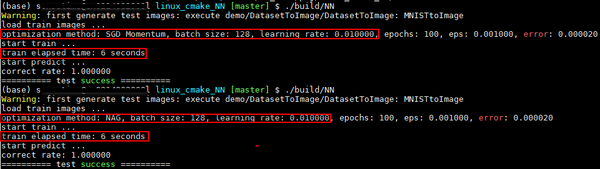
       执行结果如下图所示：测试函数为test_logistic_regression2_gradient_descent，多次执行每种配置，最终结果都相同。图像集使用MNIST，其中训练图像总共10000张，0和1各5000张，均来自于训练集；预测图像总共1800张，0和1各900张，均来自于测试集。NAG和Momentum SGD配置参数相同的情况下，即学习率为0.01，动量设为0.7，它们的耗时均为6秒，识别率均为100%

       GitHub：https://github.com/fengbingchun/NN_Test