1. 最小二乘法
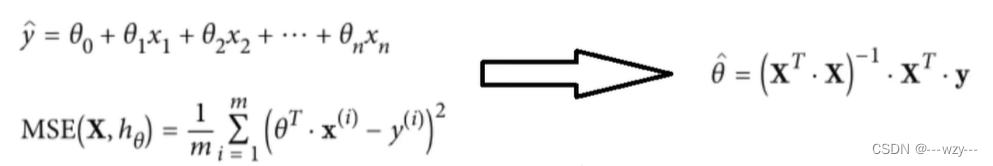
上述方法可以直接得到线性回归方程
import numpy as np
import matplotlib.pyplot as plt
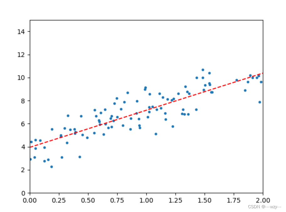
x=2*np.random.rand(100,1)
y=4+3*x+np.random.randn(100,1)
plt.plot(x,y,'.')
x=np.c_[np.ones((100,1)),x]
#公式
theta=np.linalg.inv(x.T.dot(x)).dot(x.T).dot(y)
test_x=np.array([[0],[2]])
test_x_b=np.c_[np.ones((2,1)),test_x]
predict_y=test_x_b.dot(theta)
plt.plot(test_x,predict_y,'r--')
plt.axis([0,2,0,15])
plt.show()
2.通过sklearn库函数
from sklearn.linear_model import LinearRegression
import numpy as np
x=2*np.random.rand(100,1)
y=4+3*x+np.random.randn(100,1)
lin_reg=LinearRegression()
lin_reg.fit(x,y)
#获取theta
print(lin_reg.coef_)
#获取偏置值
print(lin_reg.intercept_)
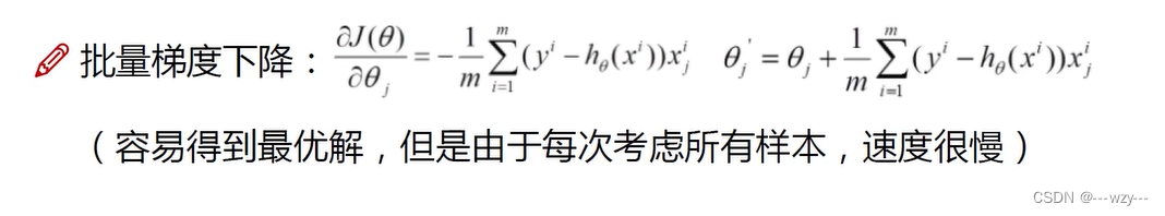
3.批量梯度下降
import numpy as np
x=2*np.random.rand(100,1)
y=4+3*x+np.random.randn(100,1)
learning_rate=0.01
iterations=1000
x_b=np.c_[np.ones((100,1)),x]
m=100
theta=np.random.randn(2,1)
for i in range(iterations):  #迭代次数
    gradients=2/m*(x_b).T.dot(x_b.dot(theta)-y)
    theta=theta-learning_rate*gradients
print(theta)
4.随机梯度下降
import numpy as np
x=2*np.random.rand(100,1)
y=4+3*x+np.random.randn(100,1)
x_b=np.c_[np.ones((x.shape[0],1)),x];
n_epochs=50
m=x_b.shape[0]
theta=np.random.randn(2,1)
learning_rate=0.01
for epoch in range(n_epochs):   #迭代次数
    for i in range(m):          #每次迭代过程中随机选择样本优化的次数
        random_index=np.random.randint(m)
        xi=x_b[random_index:random_index+1]
        yi=y[random_index:random_index+1]
        gradients=2*xi.T.dot(xi.dot(theta)-yi)
        theta=theta-learning_rate*gradients
print(theta)
5.小批量梯度下降
import numpy as np
x=2*np.random.rand(100,1)
y=4+3*x+np.random.randn(100,1)
x_b=np.c_[np.ones((x.shape[0],1)),x];
n_epochs=50     #迭代次数
minibatch=16    #小批量处理的个数
m=x_b.shape[0]
learing_rate=0.01
theta=np.random.randn(2,1)
for epoch in range(n_epochs):
    shuffled_indices=np.random.permutation(m)  #每次迭代中打乱下标,这样每次迭代按顺序选取的样本不同
    x_b_shuffled=x_b[shuffled_indices]
    y_shuffled=y[shuffled_indices]
    for i in range(0,m,minibatch):
        xi=x_b_shuffled[i:i+minibatch]
        yi=y_shuffled[i:i+minibatch]
        gradients=2/minibatch*xi.T.dot(xi.dot(theta)-yi)
        theta=theta-learing_rate*gradients
print(theta)
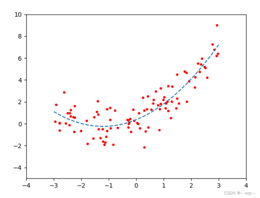
6.多元线性回归
import numpy as np
import matplotlib.pyplot as plt
from sklearn.preprocessing import PolynomialFeatures
from sklearn.linear_model import LinearRegression
x=6*np.random.rand(100,1)-3
y=0.5*x**2+x+np.random.randn(100,1)
plt.plot(x,y,'r.')
plt.axis([-4,4,-5,10])
ploy=PolynomialFeatures(degree=2,include_bias=False)
#将x变成含有x,x^2,degree为要添加的维度,include_bias为是否添加偏置项
x_ploy=ploy.fit_transform(x)
print(x[0])
print(x_ploy[0])
"""
[-2.84058046]
[-2.84058046  8.06889736]
"""
lin_reg=LinearRegression()
lin_reg.fit(x_ploy,y)
print(lin_reg.coef_)
print(lin_reg.intercept_)
"""
[[0.99806951 0.49324959]]
[-0.02205689]
"""
x_pred=np.linspace(-3,3,100).reshape(100,1)
x_pred_ploy=ploy.transform(x_pred)
y_pred=lin_reg.predict(x_pred_ploy)
plt.plot(x_pred,y_pred,'--')
plt.show()
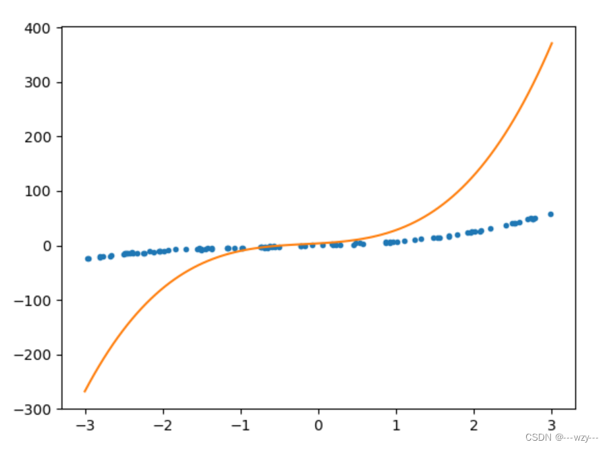
6.建立流水化
from sklearn.pipeline import Pipeline
from sklearn.preprocessing import StandardScaler
from sklearn.preprocessing import PolynomialFeatures
from sklearn.linear_model import LinearRegression
import numpy as np
import matplotlib.pyplot as plt
x=6*np.random.rand(100,1)-3
y=x**3+2*x**2+x*5+np.random.randn(100,1)
plt.plot(x,y,'.')
poly=PolynomialFeatures(degree=3,include_bias=False)   #实例出转化维度的对象
std=StandardScaler()                                   #标准化
lin_reg=LinearRegression()                             #线性回归
polynomial_reg=Pipeline([('poly_features',poly),
                         ('StandardScaler',std),
                         ('lin_reg',lin_reg)])
#该类会依次调用前面函数的fit()和transfrom()函数,只调用最后一个函数的fit()函数
polynomial_reg.fit(x,y)
print(lin_reg.coef_)
print(lin_reg.intercept_)
x_test=np.linspace(-3,3,100).reshape(100,1)
x_test_p=poly.transform(x_test)
y_test=lin_reg.predict(x_test_p)
plt.plot(x_test,y_test)
plt.show()
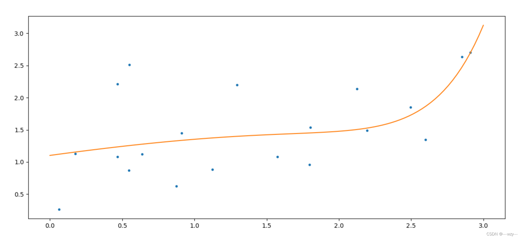
7.正则化------岭回归
α表示正则化系数

from sklearn.pipeline import Pipeline
from sklearn.preprocessing import StandardScaler
from sklearn.preprocessing import PolynomialFeatures
from sklearn.linear_model import Ridge
import numpy as np
import matplotlib.pyplot as plt
plt.figure(figsize=(14,6))
np.random.seed(42)
x=3*np.random.rand(20,1)
y=0.5*x+np.random.randn(20,1)/1.5+1
plt.plot(x,y,'.')
poly=PolynomialFeatures(degree=10,include_bias=False)
std=StandardScaler()
lin_reg=Ridge(alpha=0.5)
#正则化系数,正则化系数越大,表示theta越平均,即函数曲线越平
polynomial_reg=Pipeline([('poly_features',poly),
                         ('StandardScaler',std),
                         ('lin_reg',lin_reg)])
polynomial_reg.fit(x,y)
x_test=np.linspace(0,3,100).reshape(100,1)
x_test_p=poly.transform(x_test)
y_test=polynomial_reg.predict(x_test)
plt.plot(x_test,y_test)
plt.show()
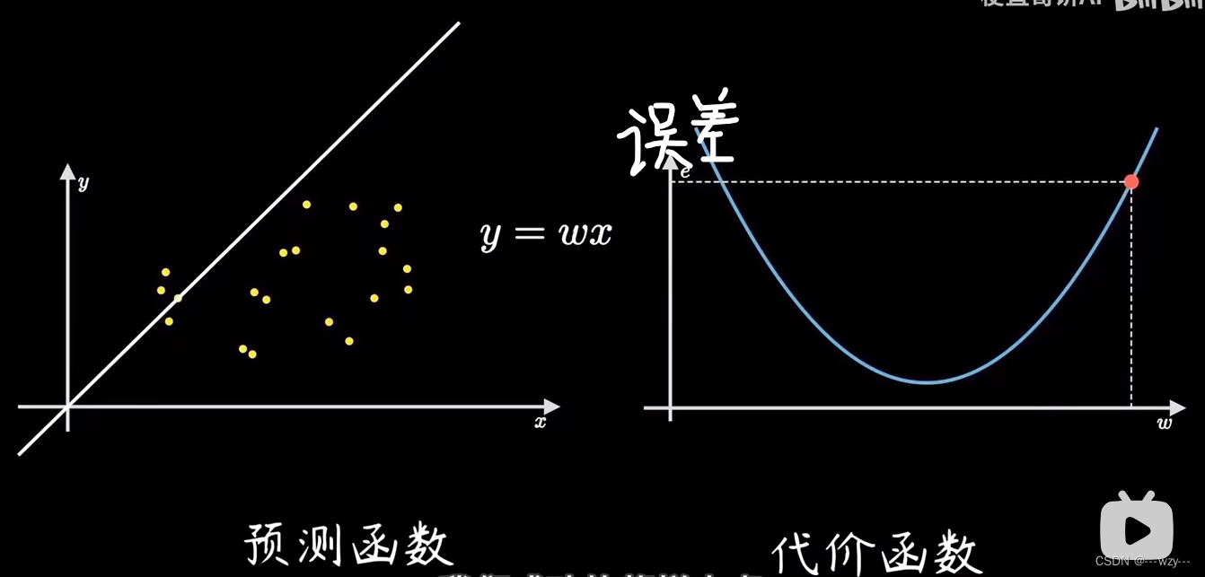
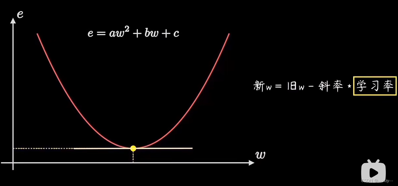
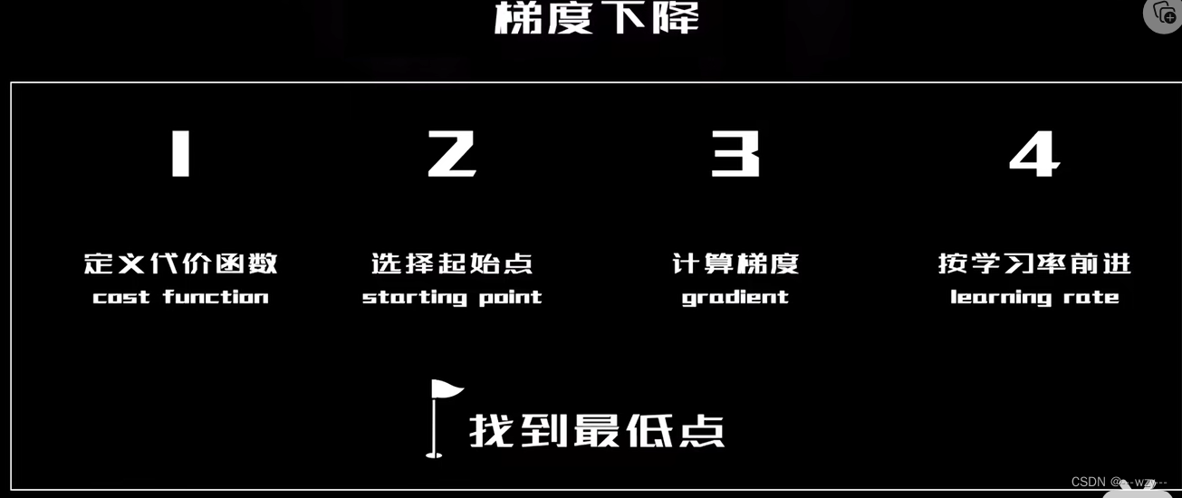
梯度下降含义
在线性回归问题中,误差函数是一个开口向上的二次函数
建立训练以及测试数据集
from sklearn.model_selection import train_test_split
import pandas as pd
data=pd.read_excel("")
X=data[:,0]
y=data[:,1]
#训练数据集0.8,测试数据集0.2
X_train,X_test,y_train,y_test=train_test_split(X,y,train_size=0.8)
#或者:X_train,X_test,y_train,y_test=train_test_split(X,y,test_size=0.2)