使用pytorch训练DCGAN(代码解析)
上一篇:使用pytorch训练DCGAN----壹
这里我使用的代码时pytorch官方提供的源码,然后根据DCGAN原论文分板块分析
板块一
导包
from __future__ import print_function
#%matplotlib inline
import argparse
import os
import random
import torch
import torch.nn as nn
import torch.nn.parallel
import torch.backends.cudnn as cudnn
import torch.optim as optim
import torch.utils.data
import torchvision.datasets as dset
import torchvision.transforms as transforms
import torchvision.utils as vutils
import numpy as np
import matplotlib.pyplot as plt
import matplotlib.animation as animation
from IPython.display import HTML

# Set random seed for reproducibility
manualSeed = 999
#manualSeed = random.randint(1, 10000) # use if you want new results
print("Random Seed: ", manualSeed)
random.seed(manualSeed)
torch.manual_seed(manualSeed)
板块二
输入参数定义
# Root directory for dataset
dataroot = "data/celeba"    # 存放数据集根目录的路径

# Number of workers for dataloader
workers = 2                 # 使用DataLoader加载数据的工作线程数

# Batch size during training
batch_size = 128            # 训练中使用的batch大小。在DCGAN论文中batch的大小为128

# Spatial size of training images. All images will be resized to this
#   size using a transformer.
image_size = 64             # 用于训练的图像的空间大小

# Number of channels in the training images. For color images this is 3
nc = 3                      # 输入图像中的颜色通道数(R-G-B)

# Size of z latent vector (i.e. size of generator input)
nz = 100                    # 潜在向量的长度

# Size of feature maps in generator
ngf = 64                    # 与通过生成器携带的特征图的深度有关

# Size of feature maps in discriminator
ndf = 64                    # 设置通过判别器传播的特征映射的深度

# Number of training epochs
num_epochs = 5              # 要运行的训练的epoch数量
# Learning rate for optimizers
lr = 0.0002                 # 学习速率。如DCGAN论文中所述,此数字应为0.0002

# Beta1 hyperparam for Adam optimizers
beta1 = 0.5                 # 适用于Adam优化器的beta1超参数。如论文所述,此数字应为0.5

# Number of GPUs available. Use 0 for CPU mode.
ngpu = 1                    # 可用的GPU数量
看似简单但这里需要注意的地方就多了,我们来看原DCGAN论文中的描述
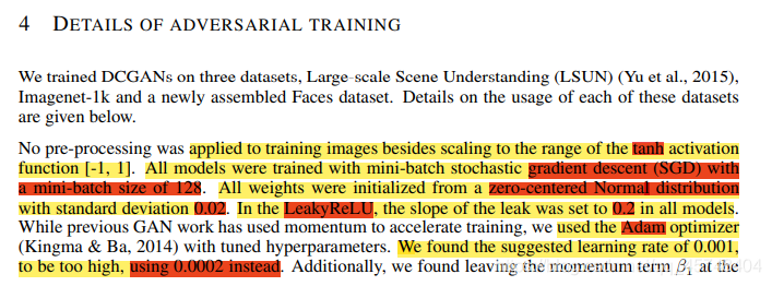
1.训练图像放缩到tanh激活函数的[-1,1]范围之内。
2.所有的模型都是通过小批量随机梯度下降法来训练的,小批量的大小是128。
3.所有的权重的初始化都是均值为0,标准差为0.02的正态分布。
4.在LeakyReLU激活函数中,所有模型的leaky的斜率都设置为0.2。
5.先前的GAN工作使用momentum来加速训练,DCGAN使用Adam optimizer来调节超参数。
6.我们发现建议使用学习速率为0.001太高了,替换为0.0002。
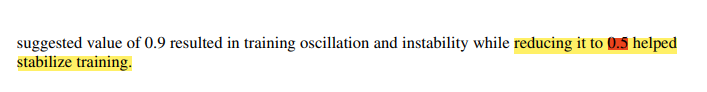
7.此外,我们发现,将momentum term β1保持在建议值0.9,会导致训练震荡和不稳定,将其减少至0.5可以帮助稳定训练
板块三
准备工作(数据集)
# We can use an image folder dataset the way we have it setup.
# Create the dataset
dataset = dset.ImageFolder(root=dataroot,
                           transform=transforms.Compose([
                               transforms.Resize(image_size),
                               transforms.CenterCrop(image_size),
                               transforms.ToTensor(),
                               transforms.Normalize((0.5, 0.5, 0.5), (0.5, 0.5, 0.5)),
                           ]))
# Create the dataloader
dataloader = torch.utils.data.DataLoader(dataset, batch_size=batch_size,
                                         shuffle=True, num_workers=workers)

# Decide which device we want to run on
device = torch.device("cuda:0" if (torch.cuda.is_available() and ngpu > 0) else "cpu")

# Plot some training images
real_batch = next(iter(dataloader))
plt.figure(figsize=(8,8))
plt.axis("off")
plt.title("Training Images")
plt.imshow(np.transpose(vutils.make_grid(real_batch[0].to(device)[:64], padding=2, normalize=True).cpu(),(1,2,0)))
这里需要注意的是如下代码
transform=transforms.Compose([
							   # 将输入图像调整为给定尺寸
                               transforms.Resize(image_size),
                               # 在中心裁剪给定的图像,如果size是一个int而不是(h,w)之类的序列,则会生成一个方形的裁剪。
                               transforms.CenterCrop(image_size),
                               # 转换为张量
                               transforms.ToTensor(),
                               # 用均值和标准差对张量图像进行归一化
                               transforms.Normalize((0.5, 0.5, 0.5), (0.5, 0.5, 0.5)),
                           ])
torchvision.transforms中包含了常见的图像变换函数,使用Compose可以将它们链接在一起,包括但不限于上面几种处理方式,还包括数据增强时可用到的torchvision.transforms.RandomHorizontalFlip()水平翻转,torchvision.transforms.RandomVerticalFlip()垂直翻转etc.具体可以看这里
然后是dataloader = torch.utils.data.DataLoader(dataset, batch_size=batch_size,shuffle=True, num_workers=workers),在torch.utils.data中定义了数据加载的核心程序
# torch.utils.data.DataLoader类的参数
DataLoader(
dataset,       #要从中加载数据的数据集
batch_size=1,  #每个批次要加载多少个样本,默认值:1
shuffle=False, #在每个时期重新随机播放数据,默认值:False
sampler=None,  #定义从数据集中抽取样本的策略
batch_sampler=None,#类似sampler,但是一次返回一批索引
num_workers=0,     #要用于数据加载的子进程数
collate_fn=None,   #合并样本列表以形成张量的小批量
pin_memory=False,  #数据加载器在将张量返回之前将其复制到CUDA固定的内存中
drop_last=False,   #删除最后一个不完整的批次,如果该数据集的大小不能被该批次的大小整除
timeout=0,         #收集批次的超时值
worker_init_fn=None,
*,
prefetch_factor=2,#预先加载的样本数
persistent_workers=False#使Worker Dataset实例保持活动状态
)
最后是device = torch.device("cuda:0" if (torch.cuda.is_available() and ngpu > 0) else "cpu")这一小段,当然这很容易就可以看出是判断把device放到GPU上还是CPU上。
板块四
权值初始化
# custom weights initialization called on netG and netD
def weights_init(m):
    classname = m.__class__.__name__
    if classname.find('Conv') != -1:
        nn.init.normal_(m.weight.data, 0.0, 0.02)
    elif classname.find('BatchNorm') != -1:
        nn.init.normal_(m.weight.data, 1.0, 0.02)
        nn.init.constant_(m.bias.data, 0)
这里m.__class__.__name__ 获得nn.module的名字,然后对其遍历找到对应的初始化方式,当然方法还有很多
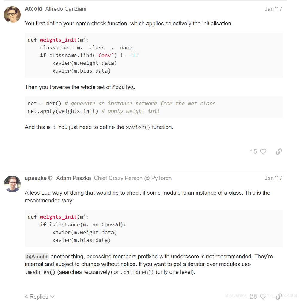
具体可以看pytorch论坛官方上对weight-initilzation的讨论
板块五
生成器
先看DCGAN原论文中的生成器模型
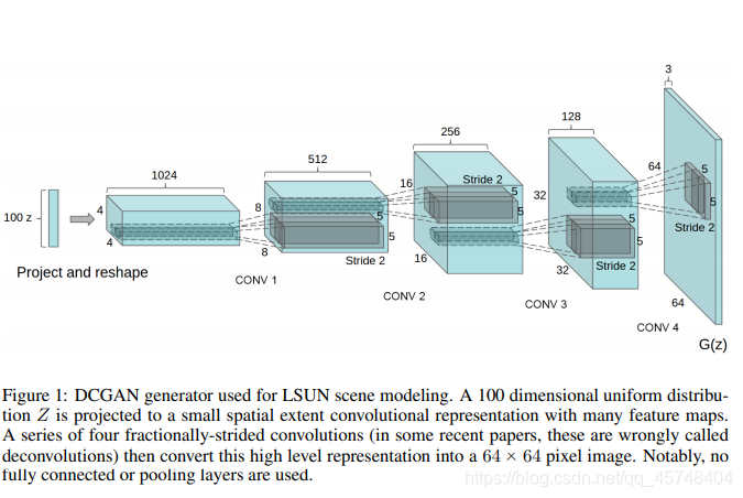
一个100维度的均匀分布z映射到一个有很多特征映射的小空间范围卷积。 四个跨步的二维卷积转置层将高层表征转换为64*64像素的图像,值得注意的是在转换层之后存在批量范数函数,这是DCGAN论文的关键贡献。
# Generator Code

class Generator(nn.Module):
    def __init__(self, ngpu):
        super(Generator, self).__init__()
        self.ngpu = ngpu
        self.main = nn.Sequential( # 顺序容器
            # input is Z, going into a convolution
            nn.ConvTranspose2d( nz, ngf * 8, 4, 1, 0, bias=False),    #转置卷积
            nn.BatchNorm2d(ngf * 8),                                  #BN层
            nn.ReLU(True),                                            #ReLu激活
            # state size. (ngf*8) x 4 x 4
            nn.ConvTranspose2d(ngf * 8, ngf * 4, 4, 2, 1, bias=False),#转置卷积
            nn.BatchNorm2d(ngf * 4),                                  #BN层
            nn.ReLU(True),                                            #ReLu激活
            # state size. (ngf*4) x 8 x 8
            nn.ConvTranspose2d( ngf * 4, ngf * 2, 4, 2, 1, bias=False),
            nn.BatchNorm2d(ngf * 2),
            nn.ReLU(True),
            # state size. (ngf*2) x 16 x 16
            nn.ConvTranspose2d( ngf * 2, ngf, 4, 2, 1, bias=False),
            nn.BatchNorm2d(ngf),
            nn.ReLU(True),
            # state size. (ngf) x 32 x 32
            nn.ConvTranspose2d( ngf, nc, 4, 2, 1, bias=False),        #转置卷积
            nn.Tanh()                                                 #Tanh
            # state size. (nc) x 64 x 64
        )

    def forward(self, input):
        return self.main(input)
构建自己的网络需要自己定义torch.nn.Module的一个子类,重写初始化函数__init__()和前向过程forward(),需要注意的是初始化时用的时torch.nn中的方法不是torch.nn.functional中的方法。
torch. nn.Module中实现layer的都是一个特殊的类,可以去查阅,他们都是以class xxxx来定义的, 会自动提取可学习的参数
nn.functional中的函数,更像是纯函数,由def function( )定义,只是进行简单的 数学运算而已。
说到这里你可能就明白二者的区别了,functional中的函数是一个确定的不变的运算公式,输入数据产生输出就ok。
然后注意到在init时定义了个main其中顺序定义(nn.Sequential)网络结构然后在forward中调用main,思路清晰代码简洁(我觉得)。
# Create the generator
netG = Generator(ngpu).to(device) # 实例化一个生成器并把它放到device中去

# Handle multi-gpu if desired
if (device.type == 'cuda') and (ngpu > 1):
    netG = nn.DataParallel(netG, list(range(ngpu)))

# Apply the weights_init function to randomly initialize all weights
#  to mean=0, stdev=0.2.
netG.apply(weights_init) # 递归的调用weights_init函数,遍历netG的submodule作为参数

# Print the model
print(netG)
得到结果
Generator(
(main): Sequential(
(0): ConvTranspose2d(100, 512, kernel_size=(4, 4), stride=(1, 1), bias=False)
(1): BatchNorm2d(512, eps=1e-05, momentum=0.1, affine=True, track_running_stats=True)
(2): ReLU(inplace=True)
(3): ConvTranspose2d(512, 256, kernel_size=(4, 4), stride=(2, 2), padding=(1, 1), bias=False)
(4): BatchNorm2d(256, eps=1e-05, momentum=0.1, affine=True, track_running_stats=True)
(5): ReLU(inplace=True)
(6): ConvTranspose2d(256, 128, kernel_size=(4, 4), stride=(2, 2), padding=(1, 1), bias=False)
(7): BatchNorm2d(128, eps=1e-05, momentum=0.1, affine=True, track_running_stats=True)
(8): ReLU(inplace=True)
(9): ConvTranspose2d(128, 64, kernel_size=(4, 4), stride=(2, 2), padding=(1, 1), bias=False)
(10): BatchNorm2d(64, eps=1e-05, momentum=0.1, affine=True, track_running_stats=True)
(11): ReLU(inplace=True)
(12): ConvTranspose2d(64, 3, kernel_size=(4, 4), stride=(2, 2), padding=(1, 1), bias=False)
(13): Tanh()
)
)
板块六
判别器
class Discriminator(nn.Module):
    def __init__(self, ngpu):
        super(Discriminator, self).__init__()
        self.ngpu = ngpu
        self.main = nn.Sequential(
            # input is (nc) x 64 x 64
            nn.Conv2d(nc, ndf, 4, 2, 1, bias=False),         #卷积层
            nn.LeakyReLU(0.2, inplace=True),                 #原文使用LeakyReLU且斜率为0.2
            # state size. (ndf) x 32 x 32
            nn.Conv2d(ndf, ndf * 2, 4, 2, 1, bias=False),
            nn.BatchNorm2d(ndf * 2),
            nn.LeakyReLU(0.2, inplace=True),
            # state size. (ndf*2) x 16 x 16
            nn.Conv2d(ndf * 2, ndf * 4, 4, 2, 1, bias=False),
            nn.BatchNorm2d(ndf * 4),
            nn.LeakyReLU(0.2, inplace=True),
            # state size. (ndf*4) x 8 x 8
            nn.Conv2d(ndf * 4, ndf * 8, 4, 2, 1, bias=False),
            nn.BatchNorm2d(ndf * 8),
            nn.LeakyReLU(0.2, inplace=True),
            # state size. (ndf*8) x 4 x 4
            nn.Conv2d(ndf * 8, 1, 4, 1, 0, bias=False),
            nn.Sigmoid()                                     #sigmoid函数
        )

    def forward(self, input):
        return self.main(input)
这里同上
# Create the Discriminator
netD = Discriminator(ngpu).to(device)

# Handle multi-gpu if desired
if (device.type == 'cuda') and (ngpu > 1):
    netD = nn.DataParallel(netD, list(range(ngpu)))

# Apply the weights_init function to randomly initialize all weights
#  to mean=0, stdev=0.2.
netD.apply(weights_init)

# Print the model
print(netD)
得到结果
Discriminator(
(main): Sequential(
(0): Conv2d(3, 64, kernel_size=(4, 4), stride=(2, 2), padding=(1, 1), bias=False)
(1): LeakyReLU(negative_slope=0.2, inplace=True)
(2): Conv2d(64, 128, kernel_size=(4, 4), stride=(2, 2), padding=(1, 1), bias=False)
(3): BatchNorm2d(128, eps=1e-05, momentum=0.1, affine=True, track_running_stats=True)
(4): LeakyReLU(negative_slope=0.2, inplace=True)
(5): Conv2d(128, 256, kernel_size=(4, 4), stride=(2, 2), padding=(1, 1), bias=False)
(6): BatchNorm2d(256, eps=1e-05, momentum=0.1, affine=True, track_running_stats=True)
(7): LeakyReLU(negative_slope=0.2, inplace=True)
(8): Conv2d(256, 512, kernel_size=(4, 4), stride=(2, 2), padding=(1, 1), bias=False)
(9): BatchNorm2d(512, eps=1e-05, momentum=0.1, affine=True, track_running_stats=True)
(10): LeakyReLU(negative_slope=0.2, inplace=True)
(11): Conv2d(512, 1, kernel_size=(4, 4), stride=(1, 1), bias=False)
(12): Sigmoid()
)
)
板块七
训练
# Initialize BCELoss function
criterion = nn.BCELoss()# 二进制交叉熵损失函数

# Create batch of latent vectors that we will use to visualize
#  the progression of the generator
fixed_noise = torch.randn(64, nz, 1, 1, device=device)

# Establish convention for real and fake labels during training
real_label = 1.#真实标签
fake_label = 0.#假标签

# Setup Adam optimizers for both G and D
optimizerD = optim.Adam(netD.parameters(), lr=lr, betas=(beta1, 0.999))
optimizerG = optim.Adam(netG.parameters(), lr=lr, betas=(beta1, 0.999))
这里需要注意的是损失函数使用的是二进制交叉熵损失函数(BCE)

设置了两个单独的优化器D和G。如DCGAN论文中所指定,这两个都是学习速度为0.0002和Beta1 = 0.5的Adam优化器
# Training Loop

# Lists to keep track of progress
img_list = []
G_losses = []
D_losses = []
iters = 0

print("Starting Training Loop...")
# For each epoch
for epoch in range(num_epochs):
    # For each batch in the dataloader
    for i, data in enumerate(dataloader, 0):

        ############################
        # (1) Update D network: maximize log(D(x)) + log(1 - D(G(z)))
        ###########################
        ## Train with all-real batch
        netD.zero_grad()
        # Format batch
        real_cpu = data[0].to(device)
        b_size = real_cpu.size(0)
        label = torch.full((b_size,), real_label, dtype=torch.float, device=device)
        # Forward pass real batch through D
        output = netD(real_cpu).view(-1)
        # Calculate loss on all-real batch
        errD_real = criterion(output, label)
        # Calculate gradients for D in backward pass
        errD_real.backward()
        D_x = output.mean().item()

        ## Train with all-fake batch
        # Generate batch of latent vectors
        noise = torch.randn(b_size, nz, 1, 1, device=device)
        # Generate fake image batch with G
        fake = netG(noise)
        label.fill_(fake_label)
        # Classify all fake batch with D
        output = netD(fake.detach()).view(-1)
        # Calculate D's loss on the all-fake batch
        errD_fake = criterion(output, label)
        # Calculate the gradients for this batch
        errD_fake.backward()
        D_G_z1 = output.mean().item()
        # Add the gradients from the all-real and all-fake batches
        errD = errD_real + errD_fake                    #损失是真实值的损失和生成值损失之和
        # Update D
        optimizerD.step()

        ############################
        # (2) Update G network: maximize log(D(G(z)))
        ###########################
        netG.zero_grad()
        label.fill_(real_label)  # fake labels are real for generator cost
        # Since we just updated D, perform another forward pass of all-fake batch through D
        output = netD(fake).view(-1)
        # Calculate G's loss based on this output
        errG = criterion(output, label)
        # Calculate gradients for G
        errG.backward()
        D_G_z2 = output.mean().item()
        # Update G
        optimizerG.step()

        # Output training stats
        if i % 50 == 0:
            print('[%d/%d][%d/%d]\tLoss_D: %.4f\tLoss_G: %.4f\tD(x): %.4f\tD(G(z)): %.4f / %.4f'
                  % (epoch, num_epochs, i, len(dataloader),
                     errD.item(), errG.item(), D_x, D_G_z1, D_G_z2))

        # Save Losses for plotting later
        G_losses.append(errG.item())
        D_losses.append(errD.item())

        # Check how the generator is doing by saving G's output on fixed_noise
        if (iters % 500 == 0) or ((epoch == num_epochs-1) and (i == len(dataloader)-1)):
            with torch.no_grad():
                fake = netG(fixed_noise).detach().cpu()
            img_list.append(vutils.make_grid(fake, padding=2, normalize=True))

        iters += 1
第1部分-训练辨别器
训练鉴别器的目的是最大程度地提高将给定输入正确分类为真实或伪造的可能性
实际上,我们想最大化 log(D(x))+log(1−D(G(z)))
首先,我们将从训练集中构造一批真实样本,向前传递D,计算损失(log(D(x)))
然后在向后传递中计算梯度
其次,我们将使用生成器构造一批假样品,将这批假样品通过D,计算损失(log(1−D(G(z)))),并通过向后传递来累积梯度
第2部分-训练生成器
如原始论文所述,我们希望通过最小化训练生成器最小化log(1−D(G(z)))产生更好的假样品即我们希望最大化log(D(G(z)))。
在代码中,通过以下方式实现此目的:使用辨别器对第1部分中的生成器输出进行分类,使用真实标签作为GT计算G的损失,计算G的梯度,最后通过优化步骤更新G的参数。将真实标签用作损失函数的GT标签似乎违反直觉,但这允许我们使用 log(x) BCELoss的一部分(而不是 log(1−x) 部分)正是我们想要的。
然后需要注意的是pytorch中训练的一般步骤
for input, target in dataset:
    optimizer.zero_grad()         # 梯度归零
    output = model(input)         # 向前传播的到结果
    loss = loss_fn(output, target)# 计算损失
    loss.backward()               # 反向传播
    optimizer.step()              # 更新参数
其次是如mean(),item(),,full(),vew(-1)(-1为自动推断)等基本操作。
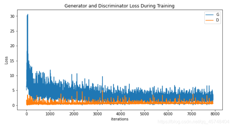
最后是展示部分
plt.figure(figsize=(10,5))
plt.title("Generator and Discriminator Loss During Training")
plt.plot(G_losses,label="G")
plt.plot(D_losses,label="D")
plt.xlabel("iterations")
plt.ylabel("Loss")
plt.legend()
plt.show()
#%%capture
fig = plt.figure(figsize=(8,8))
plt.axis("off")
ims = [[plt.imshow(np.transpose(i,(1,2,0)), animated=True)] for i in img_list]
ani = animation.ArtistAnimation(fig, ims, interval=1000, repeat_delay=1000, blit=True)

HTML(ani.to_jshtml())
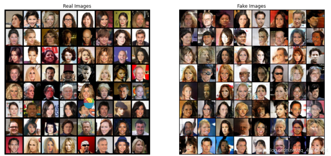
# Grab a batch of real images from the dataloader
real_batch = next(iter(dataloader))

# Plot the real images
plt.figure(figsize=(15,15))
plt.subplot(1,2,1)
plt.axis("off")
plt.title("Real Images")
plt.imshow(np.transpose(vutils.make_grid(real_batch[0].to(device)[:64], padding=5, normalize=True).cpu(),(1,2,0)))

# Plot the fake images from the last epoch
plt.subplot(1,2,2)
plt.axis("off")
plt.title("Fake Images")
plt.imshow(np.transpose(img_list[-1],(1,2,0)))
plt.show()