人工智能
第四章 分类模型
一、分类业务模型
- 分类预测模型与回归不同,回归模型是根据已知的输入和输出寻找一个性能最佳的模型,从而通过未知输出的样本得到连续的输出;而分类模型则是需要得到离散的输出,即根据已知样本的所属类别预测未知输出的样本所属的类别。
- 例如:根据工作经验预测薪资级别。
二、鸢尾花数据集数据分析
- 分析鸢尾花数据集特征。
- 基于 sklearn.datasets 加载鸢尾花数据集
- 数据集特征可视化分析
import numpy as np
import pandas as pd
import matplotlib.pyplot as plt
import sklearn.datasets as sd
iris = sd.load_iris()
iris.keys()
"""
dict_keys(['data', 'target', 'frame', 'target_names', 'DESCR', 'feature_names', 'filename', 'data_module'])
"""
print(iris.DESCR)
"""
.. _iris_dataset:
Iris plants dataset
--------------------
**Data Set Characteristics:**
# 样本数量:150,每个类别有50个样本
:Number of Instances: 150 (50 in each of three classes)
# 属性数量:4列
:Number of Attributes: 4 numeric, predictive attributes and the class
:Attribute Information:
# 萼片长度,宽度
- sepal length in cm
- sepal width in cm
# 花瓣长度,宽度
- petal length in cm
- petal width in cm
- class:
- Iris-Setosa
- Iris-Versicolour
- Iris-Virginica
:Summary Statistics:
============== ==== ==== ======= ===== ====================
Min Max Mean SD Class Correlation
============== ==== ==== ======= ===== ====================
sepal length: 4.3 7.9 5.84 0.83 0.7826
sepal width: 2.0 4.4 3.05 0.43 -0.4194
petal length: 1.0 6.9 3.76 1.76 0.9490 (high!)
petal width: 0.1 2.5 1.20 0.76 0.9565 (high!)
============== ==== ==== ======= ===== ====================
:Missing Attribute Values: None
:Class Distribution: 33.3% for each of 3 classes.
:Creator: R.A. Fisher
:Donor: Michael Marshall (MARSHALL%PLU@io.arc.nasa.gov)
:Date: July, 1988
The famous Iris database, first used by Sir R.A. Fisher. The dataset is taken
from Fisher's paper. Note that it's the same as in R, but not as in the UCI
Machine Learning Repository, which has two wrong data points.
This is perhaps the best known database to be found in the
pattern recognition literature. Fisher's paper is a classic in the field and
is referenced frequently to this day. (See Duda & Hart, for example.) The
data set contains 3 classes of 50 instances each, where each class refers to a
type of iris plant. One class is linearly separable from the other 2; the
latter are NOT linearly separable from each other.
.. topic:: References
- Fisher, R.A. "The use of multiple measurements in taxonomic problems"
Annual Eugenics, 7, Part II, 179-188 (1936); also in "Contributions to
Mathematical Statistics" (John Wiley, NY, 1950).
- Duda, R.O., & Hart, P.E. (1973) Pattern Classification and Scene Analysis.
(Q327.D83) John Wiley & Sons. ISBN 0-471-22361-1. See page 218.
- Dasarathy, B.V. (1980) "Nosing Around the Neighborhood: A New System
Structure and Classification Rule for Recognition in Partially Exposed
Environments". IEEE Transactions on Pattern Analysis and Machine
Intelligence, Vol. PAMI-2, No. 1, 67-71.
- Gates, G.W. (1972) "The Reduced Nearest Neighbor Rule". IEEE Transactions
on Information Theory, May 1972, 431-433.
- See also: 1988 MLC Proceedings, 54-64. Cheeseman et al"s AUTOCLASS II
conceptual clustering system finds 3 classes in the data.
- Many, many more ...
"""
iris.target_names # 类别
"""
array(['setosa', 'versicolor', 'virginica'], dtype='<U10')
"""
iris.feature_names # 特征名称
"""
['sepal length (cm)',
'sepal width (cm)',
'petal length (cm)',
'petal width (cm)']
"""
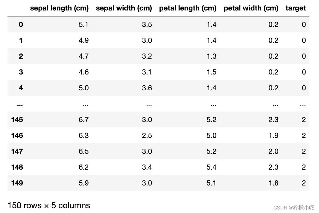
data = pd.DataFrame(iris.data, columns=iris.feature_names)
data['target'] = iris.target
data
# 基于透视表完成简单数据统计分析
data.pivot_table(index='target')
"""
		petal length (cm)	petal width (cm)	sepal length (cm)	sepal width (cm)
target
0		1.462				0.246				5.006				3.428
1		4.260				1.326				5.936				2.770
2		5.552				2.026				6.588				2.974
"""
# 可视化 花瓣的长和宽
data.plot.scatter(x='petal length (cm)', y='petal width (cm)', c='target', cmap='brg', s=20) # cmap 颜色映射 s 调节点大小

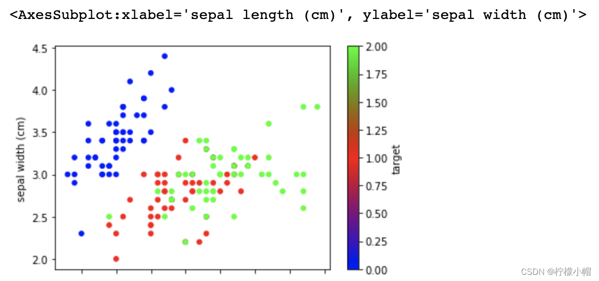
# 可视化 萼片的长和宽
data.plot.scatter(x='sepal length (cm)', y='sepal width (cm)', c='target', cmap='brg', s=20) # cmap 颜色映射 s 调节点大小
三、逻辑回归
- 逻辑回归分类模型是一种基于回归思想实现分类业务的分类模型。
- 逻辑回归做二元分类时的核心思想为:
- 针对输出为{0,1}的已知训练样本训练一个回归模型,使得训练样本的预测输出限制在(0,1)的数值区间。
- 使得原类别为0的样本的输出更接近于0,原类别为1的样本的输出更接近于1。
- 这样就可以使用相同的回归模型来完成分类预测。
- 基于回归思想来解决分类问题
- 尝试使用简单的线性模型来表达数据输入与输出的关系:
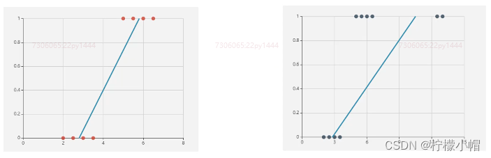
- 首先使用简单的线性模型来表达数据输入与输出的关系:
y
=
w
0
+
w
1
x
1
+
w
2
x
2
y = w_0 + w_1x_1 + w_2x_2
y=w0+w1x1+w2x2
- 然后使用逻辑函数把结果限制在(0,1)区间内:
逻
辑
函
数
(
s
i
g
m
o
i
d
)
:
y
^
=
1
1
+
e
−
y
逻辑函数(sigmoid):\hat{y} = \frac{1}{1+e^{-y}}
逻辑函数(sigmoid):y^=1+e−y1
- 所以逻辑回归的目标函数为:
y
^
=
1
1
+
e
−
(
w
0
+
w
1
x
1
+
w
2
x
2
)
\hat{y} = \frac{1}{1+e^{-(w_0 + w_1x_1 + w_2x_2)}}
y^=1+e−(w0+w1x1+w2x2)1
- 基于该目标函数,设计损失函数,求得最优模型参数使总样本预测概率误差向最小值收敛
- 逻辑回归目标函数:
逻
辑
函
数
(
s
i
g
m
o
i
d
)
:
y
^
=
1
1
+
e
−
z
;
z
=
w
T
x
+
b
逻辑函数(sigmoid):\hat{y} = \frac{1}{1+e^{-z}}; z=w^Tx +b
逻辑函数(sigmoid):y^=1+e−z1;z=wTx+b
- 该逻辑函数值域被限制在(0,1)区间,这个结果可以作为样本划分为1类别的概率:当y>0.5归为1类别;当y<0.5归为0类别。可以把训练样本数据通过线性预测模型z代入逻辑函数,找到一组最优秀的模型参数使得原本属于1类别的样本输出趋近于1;原本属于0类别的样本输出趋近于0.即将预测函数的输出看做被划分为1类别的概率,择概率大的类别作为预测结果。
1. 概述
1.1 什么是逻辑回归
- 逻辑回归(Logistic Regression) 虽然被称为回归,但其实际上是分类模型,常用于二分类。逻辑回归因其简单、可并行化、可解释强而受到广泛应用。二分类(也称为逻辑分类)是常见的分类方法,是将一批样本或数据划分到两个类别,例如一次考试,根据成绩可以分为及格、不及格两个类别,如下表所示:
| 姓名 |
成绩 |
分类 |
| Jerry |
86 |
1 |
| Tom |
98 |
1 |
| Lily |
58 |
0 |
| …… |
…… |
…… |
1.2 逻辑函数
- 逻辑回归是一种广义的线性回归,其原理是利用线性模型根据输入计算输出(线性模型输出值为连续),并在逻辑函数作用下,将连续值转换为两个离散值(0或1),其表达式如下:
y
=
h
(
w
1
x
1
+
w
2
x
2
+
w
3
x
3
+
.
.
.
+
w
n
x
n
+
b
)
y = h(w_1x_1 + w_2x_2 + w_3x_3 + ... + w_nx_n + b)
y=h(w1x1+w2x2+w3x3+...+wnxn+b)
- 其中,括号中的部分为线性模型,计算结果在函数
h
(
)
h()
h()的作用下,做二值化转换,函数
h
(
)
h()
h()的定义为:
h
=
1
1
+
e
−
t
h= \frac{1}{1+e^{-t}}
h=1+e−t1
t
=
w
T
x
+
b
\quad t=w^Tx+b
t=wTx+b
- 该函数称为Sigmoid函数(又称逻辑函数),能将
(
−
∞
,
+
∞
)
(-\infty, +\infty)
(−∞,+∞)的值映射到
(
0
,
1
)
(0, 1)
(0,1)之间,其图像为:
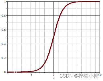
- 可以设定一个阈值(例如0.5),当函数的值大于阈值时,分类结果为1;当函数值小于阈值时,分类结果为0. 也可以根据实际情况调整这个阈值。
1.3 分类问题的损失函数
-
对于回归问题,可以使用均方差作为损失函数,对于分类问题,如何度量预测值与真实值之间的差异?分类问题采用交叉熵作为损失函数,当只有两个类别时,交叉熵表达式为:
E
(
y
,
y
^
)
=
−
[
y
l
o
g
(
y
^
)
+
(
1
−
y
)
l
o
g
(
1
−
y
^
)
]
E(y, \hat{y}) = -[y \ log(\hat{y}) + (1-y)log(1-\hat{y})]
E(y,y^)=−[y log(y^)+(1−y)log(1−y^)]
-
其中,y为真实值,
y
^
\hat{y}
y^为预测值.
- 当
y
=
1
y=1
y=1时,预测值
y
^
\hat{y}
y^越接近于1,
l
o
g
(
y
^
)
log(\hat{y})
log(y^)越接近于0,损失函数值越小,表示误差越小,预测的越准确;当预测时
y
^
\hat{y}
y^接近于0时,
l
o
g
(
y
^
)
log(\hat{y})
log(y^)接近于负无穷大,加上符号后误差越大,表示越不准确;
- 当
y
=
0
y=0
y=0时,预测值
y
^
\hat{y}
y^越接近于0,
l
o
g
(
1
−
y
^
)
log(1-\hat{y})
log(1−y^)越接近于0,损失函数值越小,表示误差越小,预测越准确;当预测值
y
^
\hat{y}
y^接近于1时,
l
o
g
(
1
−
y
^
)
log(1-\hat{y})
log(1−y^)接近于负无穷大,加上符号后误差越大,表示越不准确.
2. 逻辑回归实现
import sklearn.linear_model as lm
"""
构建逻辑回归器
solver: 用来指明损失函数的优化方法,sklearn自带了如下几种:
	liblinear:坐标轴下降法来迭代优化损失函数
	newton-cg:牛顿法的一种
	lbfgs:拟牛顿法
	sag:随机平均梯度下降(适合样本量大的情况)
penalty: 参数可选择的值为"l1"和"l2".与solver有关。
	如果是L2正则化,所有优化算法都可用。
	如果是L1正则化,只能使用“liblinear”。
C:该参数可以控制正则强度,值越小正则强度越大,可以防止过拟合。

model = lm.LogisticRegression(solver='liblinear', C=正则强度)
model.fit(训练输入集, 训练输出集)
result = model.predict(带预测输入集)
"""
# 创建模型
# solver参数:逻辑函数中指数的函数关系(liblinear表示线性关系)
# C参数:正则强度,越大拟合效果越小,通过调整该参数防止过拟合
model = lm.LogisticRegression(solver='liblinear', C=1)

# 训练
model.fit(x, y)

# 预测
pred_y = model.predict(x)
3. 二元分类实例(鸢尾花)
import sklearn.model_selection as ms
import sklearn.linear_model as lm
# 整理输入集输出集,拆分测试集训练集
x, y = sub_data.iloc[:,:-1], sub_data['target']
# 训练模型
train_x, test_x, train_y, test_y = ms.train_test_split(x, y, test_size=0.1, random_state=7)
model = lm.LogisticRegression()
model.fit(train_x, train_y)
# 评估 模型准确率
pred_test_y = model.predict(test_x)
"""
pred_test_y, test_y.values
(array([1, 1, 2, 2, 1, 1, 2, 2, 2, 1]), array([1, 1, 2, 2, 1, 1, 2, 2, 2, 1]))


print(pred_test_y==test_y)
87     True
76     True
128    True
141    True
99     True
65     True
143    True
121    True
136    True
72     True
Name: target, dtype: bool
"""
print((pred_test_y==test_y).sum() / test_y.size)
# 1.0
4. 多元分类
- 基于sigmoid函数的逻辑回归分类模型可以直接完成二元分类业务,但是若需实现多元分类则需要多个二元分类器一起工作:
| 特征1 |
特征2 |
==> |
A模型 |
B模型 |
C模型 |
| 4 |
7 |
==> |
0.7 |
0.1 |
0.2 |
| 3.5 |
8 |
==> |
0.8 |
0.1 |
0.1 |
| 1.2 |
1.9 |
==> |
0.1 |
0.6 |
0.3 |
| 5.4 |
2.2 |
==> |
0.2 |
0.1 |
0.7 |
5. 多分类实现
- 逻辑回归产生两个分类结果,可以通过多个二元分类器实现多元分类(一个多元分类问题转换为多个二元分类问题). 如有以下样本数据:
| 特征1 |
特征2 |
特征3 |
实际类别 |
|
x
1
x_1
x1 |
x
2
x_2
x2 |
x
3
x_3
x3 |
A |
|
x
1
x_1
x1 |
x
2
x_2
x2 |
x
3
x_3
x3 |
B |
|
x
1
x_1
x1 |
x
2
x_2
x2 |
x
3
x_3
x3 |
C |
-
进行以下多次分类,得到结果:
-
第一次:分为A类(值为1)和非A类(值为0)
-
第二次:分为B类(值为1)和非B类(值为0)
-
第三次:分为C类(值为1)和非C类(值为0)
-
利用逻辑分类器实现多元分类示例代码如下:
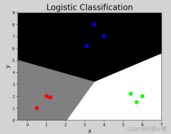
# 多元分类器示例
import numpy as np
import sklearn.linear_model as lm
import matplotlib.pyplot as mp

# 输入
x = np.array([[4, 7],
              [3.5, 8],
              [3.1, 6.2],
              [0.5, 1],
              [1, 2],
              [1.2, 1.9],
              [6, 2],
              [5.7, 1.5],
              [5.4, 2.2]])
# 输出(多个类别)
y = np.array([0, 0, 0, 1, 1, 1, 2, 2, 2])

# 创建逻辑分类器对象
model = lm.LogisticRegression(C=200) # 调整该值为1看效果
model.fit(x, y)  # 训练

# 坐标轴范围
left = x[:, 0].min() - 1
right = x[:, 0].max() + 1
h = 0.005

buttom = x[:, 1].min() - 1
top = x[:, 1].max() + 1
v = 0.005

grid_x, grid_y = np.meshgrid(np.arange(left, right, h),
                             np.arange(buttom, top, v))

mesh_x = np.column_stack((grid_x.ravel(), grid_y.ravel()))
mesh_z = model.predict(mesh_x)
mesh_z = mesh_z.reshape(grid_x.shape)

# 可视化
mp.figure('Logistic Classification', facecolor='lightgray')
mp.title('Logistic Classification', fontsize=20)
mp.xlabel('x', fontsize=14)
mp.ylabel('y', fontsize=14)
mp.tick_params(labelsize=10)
mp.pcolormesh(grid_x, grid_y, mesh_z, cmap='gray')
mp.scatter(x[:, 0], x[:, 1], c=y, cmap='brg', s=80)
mp.show()
- 执行结果:
6. 多元分类实例(鸢尾花)
import sklearn.model_selection as ms
import sklearn.linear_model as lm
# 整理输入集输出集,拆分测试集训练集
x, y = data.iloc[:,:-1], data['target']
# 训练模型
train_x, test_x, train_y, test_y = ms.train_test_split(x, y, test_size=0.1, random_state=7)
model = lm.LogisticRegression()
model.fit(train_x, train_y)
# 评估 模型准确率
pred_test_y = model.predict(test_x)
print((pred_test_y==test_y).sum() / test_y.size)
# 0.8666666666666667
7. 总结
1)逻辑回归是分类问题,用于实现二分类问题
2)实现方式:利用线性模型计算,在逻辑函数作用下产生分类
3)多分类实现:可以将多分类问题转化为二分类问题实现
4)用途:广泛用于各种分类问题
四、数据集划分
- 对于分类问题训练集和测试集的划分不应该用整个样本空间的特定百分比作为训练数据,而应该在其每一个类别的样本中抽取特定百分比作为训练数据。sklearn 模块提供了数据集划分相关方法,可以方便的划分训练集与测试集数据,使用不同数据集训练或测试模型,达到提高分类可信度。
- 数据集划分实现
import sklearn.model_selection as ms

训练输入,测试输入,训练输出,测试输出 = \
	ms.train_test_split(
		x, y, test_size=0.1, random_state=7,
		stratify=y)
import sklearn.model_selection as ms
import sklearn.linear_model as lm
# 整理输入集输出集,拆分测试集训练集
x, y = data.iloc[:,:-1], data['target']
# 训练模型
train_x, test_x, train_y, test_y = ms.train_test_split(x, y, test_size=0.1, random_state=7, stratify=y)
model = lm.LogisticRegression()
model.fit(train_x, train_y)
# 评估 模型准确率
pred_test_y = model.predict(test_x)
print((pred_test_y==test_y).sum() / test_y.size)
print(test_y.values)
"""
1.0
[2 0 0 1 0 2 2 2 1 1 2 1 1 0 0]
"""
五、交叉验证
- 由于数据集的划分有不确定性,若随机划分的样本正好处于某类特殊样本,则得到的训练模型所预测的结果的可信度将受到质疑。所以需要进行多次交叉验证,把样本空间中的所有样本均分成n份,使用不同的训练集训练模型,对不同的测试集进行测试时输出指标得分。
1. 交叉验证实现
import sklearn.model_selection as ms
指标性数组 = \
	ms.cross_val_score(模型,输入集,输出集,cv=折叠数,scoring=指标名)
import sklearn.model_selection as ms
import sklearn.linear_model as lm
# 整理输入集输出集,拆分测试集训练集
x, y = data.iloc[:,:-1], data['target']
# 训练模型
train_x, test_x, train_y, test_y = ms.train_test_split(x, y, test_size=0.1, random_state=7, stratify=y)
model = lm.LogisticRegression()
# 做5次交叉验证
scores = ms.cross_val_score(model, x, y, cv=5, scoring='accuracy')
scores.mean()
"""
0.9733333333333334
"""
model.fit(train_x, train_y)
# 评估 模型准确率
pred_test_y = model.predict(test_x)
print((pred_test_y==test_y).sum() / test_y.size)
print(test_y.values)
"""
1.0
[2 0 0 1 0 2 2 2 1 1 2 1 1 0 0]
"""
2. 交叉验证指标
- sklearn 提供的常用交叉验证指标如下:
- 精确度(accuracy) :分类正确的样本数 / 总样本数
- 查准率(precision_weighted):针对每一个类别,预测正确的样本数比上预测出来的样本数
- 召回率(recall_weighted):针对每一个类别,预测正确的样本数比上实际存在的样本数
- f1得分(f1_weighted):2 × 查准率 × 召回率 / (查准率 + 召回率)
import sklearn.model_selection as ms
import sklearn.linear_model as lm
# 整理输入集输出集,拆分测试集训练集
x, y = data.iloc[:,:-1], data['target']
# 训练模型
train_x, test_x, train_y, test_y = ms.train_test_split(x, y, test_size=0.1, random_state=7, stratify=y)
model = lm.LogisticRegression()
# 做5次交叉验证
scores = ms.cross_val_score(model, x, y, cv=5, scoring='accuracy')
print(scores.mean())
scores = ms.cross_val_score(model, x, y, cv=5, scoring='precision_weighted')
print(scores.mean())
scores = ms.cross_val_score(model, x, y, cv=5, scoring='recall_weighted')
print(scores.mean())
scores = ms.cross_val_score(model, x, y, cv=5, scoring='f1_weighted')
print(scores.mean())
"""
0.9733333333333334
0.9767676767676768
0.9733333333333334
0.973165236323131
"""
- 在交叉验证过程中,针对每一次交叉验证,计算所有类别的查准率、召回率或者f1得分,然后取各类别相应指标值的平均数,作为这一次交叉验证的评估指标,然后再将所有交叉验证的评估指标以数组的形式返回调用者。
六、混淆矩阵
- 模型训练完毕后,针对测试集数据进行测试时,可以输出预测结果的混淆矩阵观察模型性能。
|
A类别 |
B类别 |
C类别 |
| A类别 |
3 |
1 |
1 |
| B类别 |
0 |
4 |
2 |
| C类别 |
0 |
0 |
7 |
- 每一行和每一列分别对应样本输出中的每一个类别,行表示实际类别,列表示预测类别。
- 上述表格表示的含义为:A类别实际有5个样本,B类别实际有6个样本,C类别实际有7个样本;预测结果中,A类别有3个样本预测准确,另外各有1个被预测成了B和C;B类别有4个预测准确,另外2个被预测成了C类别;C类别7个全部预测准确,但有1个本属于A类别、2个本属于B类别的被预测成了C类别。
- 比较理想的混淆矩阵:
|
A类别 |
B类别 |
C类别 |
| A类别 |
5 |
0 |
0 |
| B类别 |
0 |
6 |
0 |
| C类别 |
0 |
0 |
7 |
- 上述表格表示的含义为:A类别实际有5个样本,B类别实际有6个样本,C类别实际有7个样本;预测结果中,A类别有3个样本预测准确,另外各有1个被预测成了B和C;B类别有4个预测准确,另外2个被预测成了C类别;C类别7个全部预测准确,但有1个本属于A类别、2个本属于B类别的被预测成了C类别。
- 查准率 = 主对角线上的值 / 该值所在列的和
- 召回率 = 主对角线上的值 / 该值所在行的和
- 混淆矩阵实现
import sklearn.metrics as sm
混淆矩阵 = sm.confusion_matrix(实际输出, 预测输出)
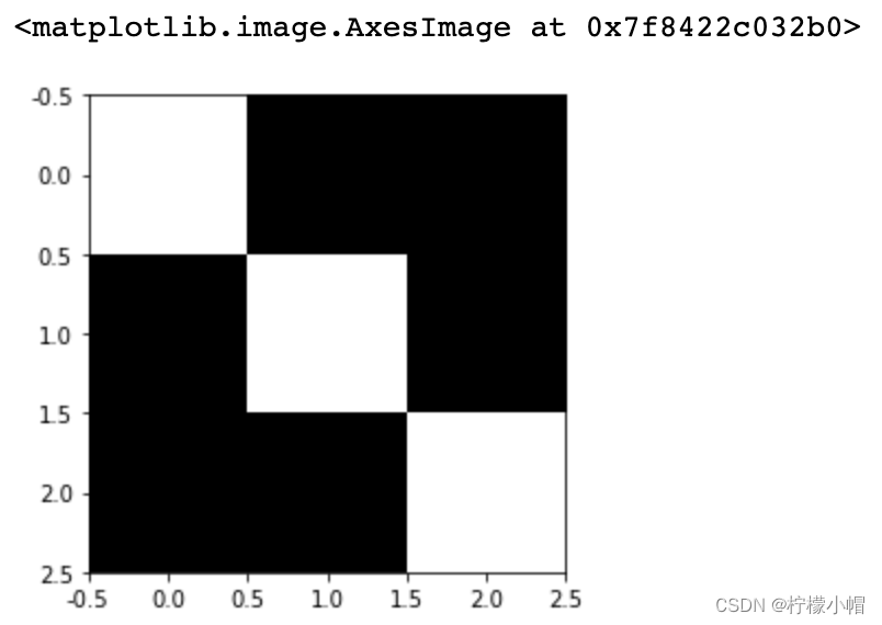
import sklearn.metrics as sm
m = sm.confusion_matrix(test_y, pred_test_y)
print(m)

"""
[[5 0 0]
 [0 5 0]
 [0 0 5]]
"""
plt.imshow(m, cmap='gray')
七、分类报告
- sklearn.metrics 提供了分类报告相关 API,不仅可以得到混淆矩阵的信息,还可以得到交叉验证查准率、召回率、f1得分的结果,可以方便的分析出哪些样本是异常样本。
- 获取模型分类结果的分类报告的相关 API:
# 获取分类报告
cr = sm.classification_report(实际输出,预测输出)
print(cr)

"""
              precision    recall  f1-score   support

           0       1.00      1.00      1.00         5
           1       1.00      1.00      1.00         5
           2       1.00      1.00      1.00         5

    accuracy                           1.00        15
   macro avg       1.00      1.00      1.00        15
weighted avg       1.00      1.00      1.00        15
"""