Secure communications: web traffic: HTTPS wireless traffic: 802.11i WPA2, GSM, Bluetooth Encrypting files on disk: EFS, TrueCrypt Content protection(e.g. DVD, Blu-ray): CSS, AACS User authentication … and much much more
Secure communication
Laptop
↔
\leftrightarrow
↔ web server protocol: HTTPS (actrual protocol: SSL/TLS)
Make sure that as this data travels across the network:
attacker can’t eavesdrop on this data
attacker can’t modify the data while it’s in the network
[no eavesdropping, no tampering]
Secure Sockets Layer/TLS
Two main parts:
Handshake Protocol: Establish shared secret key using public-key cryptography (2nd part of course)
Record Layer: Transmit data using shared secret key Ensure confidentiality and integrity (1st part of course)
Protected files on disk
attacker can’t read the contents in the file
if the attacker tries to modify the data in the file while it’s on disk, it will be detected when decrypting this file
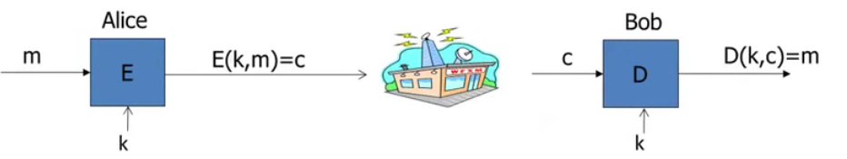
Analogous to secure communication: Alice today sends a message to Alice tomorrow.
Building block: symmetric encryption
E, D: cipher k: secret key(e.g. 128bits) m, c: plaintext, ciphertext
Encryption algorithm is publicly known Never use a proprietary cipher
Use Cases
Single use key: (one time key) Key is only used to encrypt one message e.g. encrypted email: new key generated for every email
Multi use key: (many time key) Key used to encrypt multiple messages e.g. encrypted files: same key used to encrypt many files Need more machinery than for one-time key
Things to remember
Cryptography is:
A tremendous tool
The basis for many security mechanisms
Cryptography is not:
The solution to all security problems
Reliable unless implemented and used properly
Something you should try to invest yourself many many examples of broken ad-hoc designs
What is cryptography?
Crypto core
Secret key establishment
Secure communication
But crypto cand do much more
Digital signatures
Anonymous communication
Anonymous digital cash Can I spend a “digital coin” without anyone knowing who I am? How to prevent double spending?
Protocols
Examples: -Elections -Private auctions
Secure multi-party computation
Goal: compute
f
(
x
1
,
x
2
,
x
3
,
x
4
)
f(x_1,x_2,x_3,x_4)
f(x1,x2,x3,x4) trusted authority? “Thm:” anything that can be done with a trusted authority, can also be done without a trusted authority.
Crypto magic
Privately outsourcing computation
Zero knowledge(proof of knowledge)
A rigorous science
The three steps in cryptography:
Precisely specify threat model
Propose a construction
Prove that breaking construction under threat mode will solve an underlying hard problem
History
David Kahn, “The code breakers”(1996)
Symmetric Ciphers
Few Historic Examples (all badly broken)
1. Substitution cipher
e.g. Ceaser Cipher (no key)
Q: What is the size of key space in the substitution cipher assuming 26 letters? A:
26
!
≈
2
88
26!\approx 2^{88}
26!≈288
How to break a substitution cipher?
Q: What is the most common letter in English text? A: “E”
Use frequency of English letters
Use frequency of pairs of letters (diagrams)
2. Vigener cipher (16’th century, Rome)
3. Rotor Machines (1870-1943)
Early example: the Hebern machine (single rotor) Most famous: the Enigma (3-5 rotors) # rotor positions =
2
6
4
≈
2
18
26^4\approx 2^{18}
264≈218 [total # keys =
2
36
2^{36}
236 due to optional plugboard]
U: finite set (e.g.
U
=
{
0
,
1
}
n
U=\{0, 1\}^n
U={0,1}n) Def: Probability distribution
P
P
P over
U
U
U is a function
P
:
U
→
[
0
,
1
]
P: U\rightarrow [0, 1]
P:U→[0,1] such that
∑
x
∈
U
P
(
x
)
=
1
\displaystyle\sum_{x\in U} P(x)=1
x∈U∑P(x)=1
Examples:
Uniform distribution: for all
x
∈
U
x\in U
x∈U:
P
(
x
)
=
1
/
∣
U
∣
P(x)=1/|U|
P(x)=1/∣U∣
Point distribution at
x
0
x_0
x0:
P
(
x
0
)
=
1
,
∀
x
≠
x
0
:
P
(
x
)
=
0
P(x_0)=1, \forall x\not =x_0: P(x)=0
P(x0)=1,∀x=x0:P(x)=0
Distribution vector: (Example)
(
P
(
000
)
,
P
(
001
)
,
P
(
010
)
,
.
.
.
,
P
(
111
)
)
(P(000), P(001), P(010), ..., P(111))
(P(000),P(001),P(010),...,P(111))
Event
For a set
A
⊆
U
:
P
r
[
A
]
=
∑
x
∈
A
P
(
x
)
∈
[
0
,
1
]
A\subseteq U: Pr[A]=\displaystyle\sum _{x\in A}P(x)\in [0, 1]
A⊆U:Pr[A]=x∈A∑P(x)∈[0,1]
The set
A
A
A is called an event
note:
P
r
[
U
]
=
1
Pr[U]=1
Pr[U]=1
Example:
U
=
{
0
,
1
}
8
U=\{ 0, 1\}^8
U={0,1}8
A
=
{
A=\{
A={all
x
x
x in
U
U
U that
l
s
b
2
(
x
)
=
11
}
⊆
U
lsb_2(x)=11\}\subseteq U
lsb2(x)=11}⊆U for the uniform distribution on
{
0
,
1
}
8
\{ 0, 1\}^8
{0,1}8:
P
r
[
A
]
=
1
/
4
Pr[A]=1/4
Pr[A]=1/4
[
l
s
b
2
(
x
)
=
11
lsb_2(x)=11
lsb2(x)=11: the two least significant bits of the byte is “11”]
The union bond
For events
A
1
A_1
A1 and
A
2
A_2
A2
P
r
[
A
1
∪
A
2
]
≤
P
r
[
A
1
]
+
P
r
[
A
2
]
Pr[A_1\cup A_2]\leq Pr[A_1]+Pr[A_2]
Pr[A1∪A2]≤Pr[A1]+Pr[A2]
A
1
∩
A
2
=
Φ
⟹
P
r
[
A
1
]
∪
A
2
=
P
r
[
A
1
]
+
P
r
[
A
2
]
A_1\cap A_2=\Phi \implies Pr[A_1]\cup A_2= Pr[A_1]+Pr[A_2]
A1∩A2=Φ⟹Pr[A1]∪A2=Pr[A1]+Pr[A2]
Example:
A
1
=
{
A_1=\{
A1={all
x
x
x in
{
0
,
1
}
n
\{0,1\}^n
{0,1}n s.t.
l
s
b
2
(
x
)
=
11
}
lsb_2(x)=11\}
lsb2(x)=11}
A
2
=
{
A_2=\{
A2={all
x
x
x in
{
0
,
1
}
n
\{0,1\}^n
{0,1}n s.t.
m
s
b
2
(
x
)
=
11
}
msb_2(x)=11\}
msb2(x)=11}
P
r
[
l
s
b
2
(
x
)
=
11
Pr[lsb_2(x)=11
Pr[lsb2(x)=11 or
m
s
b
2
(
x
)
=
11
]
=
P
r
[
A
1
∪
A
2
]
≤
1
/
4
+
1
/
4
=
1
/
2
msb_2(x)=11]=Pr[A_1\cup A_2]\leq 1/4+1/4=1/2
msb2(x)=11]=Pr[A1∪A2]≤1/4+1/4=1/2
[
l
s
b
2
(
x
)
=
11
lsb_2(x)=11
lsb2(x)=11: end with “11”] [
m
s
b
2
(
x
)
=
11
msb_2(x)=11
msb2(x)=11: begin with “11”]
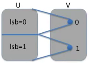
Random Variables
Def: a random variable
X
X
X is a function
X
:
U
→
V
X: U\rightarrow V
X:U→V
Example:
X
:
{
0
,
1
}
n
→
{
0
,
1
}
X: \{ 0, 1\}^n\rightarrow\{0, 1\}
X:{0,1}n→{0,1}
X
(
y
)
=
l
s
b
(
y
)
∈
{
0
,
1
}
X(y)=lsb(y)\in \{0, 1\}
X(y)=lsb(y)∈{0,1}
For the uniform distribution on
U
U
U:
P
r
[
X
=
0
]
=
1
/
2
,
P
r
[
X
=
1
]
=
1
/
2
Pr[X=0]=1/2, Pr[X=1]=1/2
Pr[X=0]=1/2,Pr[X=1]=1/2 More generally: rand.var.
X
X
X induces a distribution on
V
V
V:
P
r
[
X
=
v
]
:
=
P
r
[
X
−
1
(
v
)
]
Pr[X=v]:=Pr[X^{-1}(v)]
Pr[X=v]:=Pr[X−1(v)]
[
X
−
1
(
v
)
X^{-1}(v)
X−1(v):
a
a
a for
X
(
a
)
=
v
X(a)=v
X(a)=v] Formally we say that the probability that
X
X
X outputs
v
v
v, is the same as the probability of the event that when we sample a random element in the universe, we fall into the pre-image of
v
v
v under the function
X
X
X.
The uniform random variable
Let
U
U
U be some set, e.g.
U
=
{
0
,
1
}
n
U=\{0, 1\}^n
U={0,1}n We write
r
←
R
U
r\xleftarrow{R}U
rRU to donate a uniform random variable over
U
U
U for all
a
∈
U
a\in U
a∈U:
P
r
[
r
=
a
]
=
1
/
∣
U
∣
Pr[r=a]=1/|U|
Pr[r=a]=1/∣U∣ (formally,
r
r
r is the identity function:
r
(
x
)
=
x
r(x)=x
r(x)=x for all
x
∈
U
x\in U
x∈U)
Example: Let
r
r
r be a uniform random variable on
{
0
,
1
}
2
\{ 0, 1\}^2
{0,1}2 Define the random variable
X
=
r
1
+
r
2
X=r_1+r_2
X=r1+r2 Then
P
r
[
X
=
2
]
=
1
/
4
Pr[X=2]=1/4
Pr[X=2]=1/4
(Hint:
P
r
[
X
=
2
]
=
P
r
[
r
=
11
]
Pr[X=2]=Pr[r=11]
Pr[X=2]=Pr[r=11])
Randomized algorithms
Deterministic algorithm:
y
←
A
(
m
)
y\leftarrow A(m)
y←A(m)
Randomized algorithm:
y
←
A
(
m
;
r
)
y\leftarrow A(m;r)
y←A(m;r) where
r
←
R
{
0
,
1
}
n
r\xleftarrow{R}\{0, 1\}^n
rR{0,1}n output is a random variable
y
←
R
A
(
m
)
y\xleftarrow{R}A(m)
yRA(m)
Example:
A
(
m
;
k
)
=
E
(
k
,
m
)
A(m;k)=E(k, m)
A(m;k)=E(k,m),
y
←
R
A
(
m
)
y\xleftarrow{R}A(m)
yRA(m)
Independence
Def: events A and B independent if
P
r
[
A
Pr[A
Pr[A and
B
]
=
P
r
[
A
]
⋅
P
r
[
B
]
B]=Pr[A]\cdot Pr[B]
B]=Pr[A]⋅Pr[B] random variables X, Y taking values in V are independent if
∀
a
,
b
∈
V
:
P
r
[
X
=
a
\forall a,b\in V: Pr[X=a
∀a,b∈V:Pr[X=a and
Y
=
b
]
=
P
r
[
X
=
a
]
⋅
P
r
[
Y
=
b
]
Y=b]=Pr[X=a]\cdot Pr[Y=b]
Y=b]=Pr[X=a]⋅Pr[Y=b]
Example:
U
=
{
0
,
1
}
2
=
{
00
,
01
,
10
,
11
}
U=\{ 0, 1\}^2=\{00, 01, 10, 11\}
U={0,1}2={00,01,10,11} and
r
←
R
U
r\xleftarrow{R}U
rRU Define random variables
X
X
X and
Y
Y
Y as:
X
=
l
s
b
(
r
)
X=lsb(r)
X=lsb(r),
Y
=
m
s
b
(
r
)
Y=msb(r)
Y=msb(r)
P
r
[
X
=
0
Pr[X=0
Pr[X=0 and
Y
=
0
]
=
P
r
[
r
=
00
]
=
1
/
4
=
P
r
[
X
=
0
]
⋅
P
r
[
Y
=
0
]
Y=0]=Pr[r=00]=1/4=Pr[X=0]\cdot Pr[Y=0]
Y=0]=Pr[r=00]=1/4=Pr[X=0]⋅Pr[Y=0]
XOR
XOR of two strings in
{
0
,
1
}
n
\{ 0, 1\}^n
{0,1}n is their bit-wise addition mod 2
An important property of XOR
Y
Y
Y is a random variable over
{
0
,
1
}
n
\{ 0, 1\}^n
{0,1}n
X
X
X is a uniform random variable over
{
0
,
1
}
n
\{ 0, 1\}^n
{0,1}n
X
X
X and
Y
Y
Y are independent Then:
Z
:
=
Y
⊕
X
Z:=Y\oplus X
Z:=Y⊕X is a uniform variable on
{
0
,
1
}
n
\{ 0, 1\}^n
{0,1}n
Proof: (for n=1)
P
r
[
Z
=
0
]
=
P
r
[
(
X
,
Y
)
=
(
0
,
0
)
Pr[Z=0]=Pr[(X,Y)=(0,0)
Pr[Z=0]=Pr[(X,Y)=(0,0) or
(
X
,
Y
)
=
(
1
,
1
)
]
=
P
r
[
(
X
,
Y
)
=
(
0
,
0
)
]
⋅
P
r
[
(
X
,
Y
)
=
(
1
,
1
)
]
=
1
/
2
(X,Y)=(1,1)]=Pr[(X,Y)=(0,0)]\cdot Pr[(X,Y)=(1,1)]=1/2
(X,Y)=(1,1)]=Pr[(X,Y)=(0,0)]⋅Pr[(X,Y)=(1,1)]=1/2
The birthday paradox
Let
r
1
,
r
2
,
.
.
.
,
r
n
∈
U
r_1, r_2, ..., r_n\in U
r1,r2,...,rn∈U be independent identically distributed random variables. when
n
=
1.2
×
∣
U
∣
1
/
2
n=1.2\times |U|^{1/2}
n=1.2×∣U∣1/2 then
P
r
[
∃
i
≠
j
:
r
i
=
r
j
]
≥
1
/
2
Pr[\exist i\not = j: r_i=r_j]\geq 1/2
Pr[∃i=j:ri=rj]≥1/2 [notation:
∣
U
∣
|U|
∣U∣ is the size of
U
U
U]
Example: Let
U
=
{
0
,
1
}
128
U=\{ 0, 1\}^{128}
U={0,1}128 After sampling about
2
64
2^{64}
264 random messages from
U
U
U, some two sampled messages will likely be the same.