JPEG编码原理及文件格式及代码分析

一 JPEG编码原理
首先我们先来看一下JPEG的编码原理图

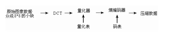
如上图所示，下面进行逐步的分析：
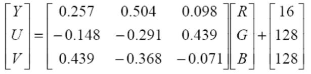
1 RGB->YUV
首先为了降低互相的关联性，将RGB转换为YUV，这样就可以对亮度信号和色度信号进行分别的处理

2 零电平偏置下移
由于后面需要对图像进行DCT变换，如果不进行偏移，会使分量值过大，所以在这里采用偏置下移的方法，便于DCT变换量化后直流的系数大大降低，也就降低了数据量。
3 分块
JPEG标准在处理图片时会先把图片分割成一个个8x8像素的方块，源图像如果不是8x8的整数倍，需进行补充，后面的DCT、量化、熵编码都是针对单个方块的操作，编码的产物是这些方块的压缩数据。压缩数据经过解码还原成像素数据，然后将一个个方块拼成一整完整图片的像素数据显示。
4 DCT变换
对每一块进行DCT变化，目的是去除图像数据之间的相关性，便于量化过程去除图像数据的空间冗余。由于人眼对图片中的低频信息（色彩变化不明显，如图片的整体色调，物体轮廓）比较敏感，对高频信息不敏感（色彩变化剧烈，如物体的边缘、人脸上的小斑点），因此我们可以利用DCT变换把图片中高频和低频部分区分开来，然后将高频部分的数据进行压缩，这样就达到压缩图片的功能。
二维DCT变换公式如下所示

需要特别强调的是，DCT是一种无损变换，这样做的目的是在为下一步的量化做准备。
５　量化
所谓量化其实就是将频率/量化步长，将量化步长以内的精度信息丢失，JPEG算法提供了两张标准的量化系数矩阵，如下所示

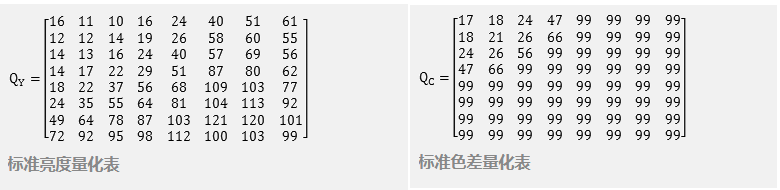
可以看出越往左上角，值越小，因此这张量化表的作用就是屏蔽高频信息。
６　压缩
在这里直流分量与交流分量采用了不同的压缩方法。
对于直流分量来说，量化后每一块所得的数值比较大，但相邻块之间的差值比较小，这就很适合采用DPCM的压缩方式，在之前的博客中有较为详细的介绍，但DPCM之后还不够，还要进行霍夫曼编码，进行进一步的压缩
对于交流分量来说，每一块中剩余的交流分量都比较小，JPEG先用RLE(run-length encoding，游程编码)编码将图像数据以“之字形”排列，如下图，这样可以尽可能的将频率为0的数据存储在一起。连续N个0，可以用一个0和一个长度N来表示，压缩效果很好，然后将剩下的位置使用霍夫曼编码。

在这里说一句，JPEG的解码就是将其编码过程倒过来，进行一步一步的还原，在这里就不细说了。
二　JPEG文件格式
JPEG文件由一系列字段组成，每个字段都有marker（标记），由0xff开头。接下来对每一个字段进行简要的说明
1　SOI
这个字段定义了文件的起始标记，标记为FFD8。
2 APP0
Application，应用程序保留标记0，标志FFE0，包含一定信息
① 数据长度 2字节 ①~⑨9个字段的总长度
即不包括标记代码，但包括本字段
② 标识符 5字节 固定值0x4A46494600，即字符串“JFIF0”
③ 版本号 2字节 一般是0x0102，表示JFIF的版本号1.2
可能会有其他数值代表其他版本
④ X和Y的密度单位 1字节 只有三个值可选
0：无单位；1：点数/英寸；2：点数/厘米
⑤ X方向像素密度 2字节 取值范围未知
⑥ Y方向像素密度 2字节 取值范围未知
⑦ 缩略图水平像素数目 1字节 取值范围未知
⑧ 缩略图垂直像素数目 1字节 取值范围未知
⑨ 缩略图RGB位图 长度可能是3的倍数 缩略图RGB位图数据
3 DQT
也就是量化表，JPEG文件一般有２个DQT段，为Y值（亮度）定义１个, 为UV值（色度）定义１个。每张量化表都由FFDB开始，量化表中的第一个字节被分成了高四位和低四位来用。高四位表示了该量化表的精度，0：8位；1：16位；低四位表示了量化表ID，取值范围为0～3；接下来是所有的表项，数量为(64×(精度+1))字节，里面都是量化的系数。量化表中的数据按照Z字形保存量化表内8x8的数据
4 SOF0
标志位FFC0，包含图像基本信息
段标识 1 FF
段类型 1 C0
段长度 2 其值＝8＋组件数量×3
　　（以下为段内容）
样本精度 1 8 每个样本位数（大多数软件不支持12和16）
图片高度 2
图片宽度 2
组件数量 1 3 1＝灰度图，3＝YCbCr/YIQ 彩色图，4＝CMYK 彩色图
　　（以下每个组件占用３字节）
组件 ID 1 1＝Y, 2＝Cb, 3＝Cr, 4＝I, 5＝Q
采样系数 1 0－3位：垂直采样系数
4－7位：水平采样系数
量化表号 1
5 DHT
标志位FFC4，存放哈夫曼表，JPEG文件里有２类Haffman 表：一类用于DC（直流量），一类用于AC（交流量）。一般有４个表：亮度的DC和AC，色度的DC和AC。最多可有６个。该Marker以FFC4作为开始标记。然后是字段长度，类型(AC/DC)，索引(Index)，位表(bit table)，值表(value table)。
6 SOS
扫描行开始，标志位FFDA，表明了字段的长度，然后说明了颜色分量数，该与SOF字段中的数据应该是保持一致的。然后针对于每一个颜色分量信息，给出了每个分量的DC/AC使用的哈夫曼表编号。
三 代码解读
本次实验主要做到了JPG文件转换为YUV文件，并且输出了量化系数以及霍夫曼码表。
首先先来看一下如何写入YUV文件，原先的代码为分别生成.Y .U .V文件，其实只需要将这三个写入的数据按照YUV的顺序写入YUV文件即可，具体代码如下所示

static void write_yuv(const char *filename, int width, int height, unsigned char **components)
{
  FILE *F;
  char temp[1024];

  snprintf(temp, 1024, "%s.Y", filename);
  F = fopen(temp, "wb");
  fwrite(components[0], width, height, F);
  fclose(F);
  snprintf(temp, 1024, "%s.U", filename);
  F = fopen(temp, "wb");
  fwrite(components[1], width*height/4, 1, F);
  fclose(F);
  snprintf(temp, 1024, "%s.V", filename);
  F = fopen(temp, "wb");
  fwrite(components[2], width*height/4, 1, F);
  fclose(F);
  snprintf(temp, 1024, "%s.YUV", filename);
  F = fopen(temp, "wb");
  fwrite(components[0], width, height, F);
  fwrite(components[1], width * height / 4, 1, F);
  fwrite(components[2], width * height / 4, 1, F);
  fclose(F);
}

结果如下所示
原图像为

生成的YUV图像为

最主要的是观看量化系数的步骤，首先先来看一下主函数中调用的convert_one_image函数

int convert_one_image(const char *infilename, const char *outfilename, int output_format)
{
  FILE *fp;
  unsigned int length_of_file;
  unsigned int width, height;
  unsigned char *buf;
  struct jdec_private *jdec;
  unsigned char *components[3];

  /* Load the Jpeg into memory */
  fp = fopen(infilename, "rb");
  if (fp == NULL)
    exitmessage("Cannot open filename\n");
  length_of_file = filesize(fp);
  buf = (unsigned char *)malloc(length_of_file + 4);
  if (buf == NULL)
    exitmessage("Not enough memory for loading file\n");
  fread(buf, length_of_file, 1, fp);
  fclose(fp);

  /* Decompress it */
  jdec = tinyjpeg_init();
  if (jdec == NULL)
    exitmessage("Not enough memory to alloc the structure need for decompressing\n");

  if (tinyjpeg_parse_header(jdec, buf, length_of_file)<0)
    exitmessage(tinyjpeg_get_errorstring(jdec));

  /* Get the size of the image */
  tinyjpeg_get_size(jdec, &width, &height);

  snprintf(error_string, sizeof(error_string),"Decoding JPEG image...\n");
  if (tinyjpeg_decode(jdec, output_format) < 0)
    exitmessage(tinyjpeg_get_errorstring(jdec));

  /* 
   * Get address for each plane (not only max 3 planes is supported), and
   * depending of the output mode, only some components will be filled 
   * RGB: 1 plane, YUV420P: 3 planes, GREY: 1 plane
   */
  tinyjpeg_get_components(jdec, components);

  /* Save it */
  switch (output_format)
   {
    case TINYJPEG_FMT_RGB24:
    case TINYJPEG_FMT_BGR24:
      write_tga(outfilename, output_format, width, height, components);
      break;
    case TINYJPEG_FMT_YUV420P:
      write_yuv(outfilename, width, height, components);
      break;
    case TINYJPEG_FMT_GREY:
      write_pgm(outfilename, width, height, components);
      break;
   }

  /* Only called this if the buffers were allocated by tinyjpeg_decode() */
  tinyjpeg_free(jdec);
  /* else called just free(jdec); */

  free(buf);
  return 0;
}

首先先读取了文件的全部信息，并用指针完成了存储，而后进行文件内容的详细读取，tinyjpeg_parse_header函数完成了对文件头部分的读取，量化表就在其中，现在让我们看看这个函数

int tinyjpeg_parse_header(struct jdec_private *priv, const unsigned char *buf, unsigned int size)
{
  int ret;

  /* Identify the file */
  if ((buf[0] != 0xFF) || (buf[1] != SOI))
    snprintf(error_string, sizeof(error_string),"Not a JPG file ?\n");

  priv->stream_begin = buf+2;
  priv->stream_length = size-2;
  priv->stream_end = priv->stream_begin + priv->stream_length;

  ret = parse_JFIF(priv, priv->stream_begin);

  return ret;
}

在这里先进行了文件格式的判断，而后开始读取里面的内容，进入parse_JFIF函数

static int parse_JFIF(struct jdec_private *priv, const unsigned char *stream)
{
  int chuck_len;
  int marker;
  int sos_marker_found = 0;
  int dht_marker_found = 0;
  const unsigned char *next_chunck;

  /* Parse marker */
  while (!sos_marker_found)
   {
     if (*stream++ != 0xff)
       goto bogus_jpeg_format;
     /* Skip any padding ff byte (this is normal) */
     while (*stream == 0xff)
       stream++;

     marker = *stream++;
     chuck_len = be16_to_cpu(stream);
     next_chunck = stream + chuck_len;
     switch (marker)
      {
       case SOF:
	 if (parse_SOF(priv, stream) < 0)
	   return -1;
	 break;
       case DQT:
	 if (parse_DQT(priv, stream) < 0)
	   return -1;
	 break;
       case SOS:
	 if (parse_SOS(priv, stream) < 0)
	   return -1;
	 sos_marker_found = 1;
	 break;
       case DHT:
	 if (parse_DHT(priv, stream) < 0)
	   return -1;
	 dht_marker_found = 1;
	 break;
       case DRI:
	 if (parse_DRI(priv, stream) < 0)
	   return -1;
	 break;
       default:
#if TRACE
	fprintf(p_trace,"> Unknown marker %2.2x\n", marker);
	fflush(p_trace);
#endif
	 break;
      }

     stream = next_chunck;
   }

  if (!dht_marker_found) {
#if TRACE
	  fprintf(p_trace,"No Huffman table loaded, using the default one\n");
	  fflush(p_trace);
#endif
    build_default_huffman_tables(priv);
  }

#ifdef SANITY_CHECK
  if (   (priv->component_infos[cY].Hfactor < priv->component_infos[cCb].Hfactor)
      || (priv->component_infos[cY].Hfactor < priv->component_infos[cCr].Hfactor))
    snprintf(error_string, sizeof(error_string),"Horizontal sampling factor for Y should be greater than horitontal sampling factor for Cb or Cr\n");
  if (   (priv->component_infos[cY].Vfactor < priv->component_infos[cCb].Vfactor)
      || (priv->component_infos[cY].Vfactor < priv->component_infos[cCr].Vfactor))
    snprintf(error_string, sizeof(error_string),"Vertical sampling factor for Y should be greater than vertical sampling factor for Cb or Cr\n");
  if (   (priv->component_infos[cCb].Hfactor!=1) 
      || (priv->component_infos[cCr].Hfactor!=1)
      || (priv->component_infos[cCb].Vfactor!=1)
      || (priv->component_infos[cCr].Vfactor!=1))
    snprintf(error_string, sizeof(error_string),"Sampling other than 1x1 for Cr and Cb is not supported");
#endif

  return 0;
bogus_jpeg_format:
#if TRACE
  fprintf(p_trace,"Bogus jpeg format\n");
  fflush(p_trace);
#endif
  return -1;
}

由上述代码可知，过程中不断读取标志位进行判断，判断结束后进行不同函数的操作，我们在这里要找量化系数，所以重点看DQT部分，也就是parse_DQT(priv, stream)这个函数

static int parse_DQT(struct jdec_private *priv, const unsigned char *stream)
{
  int qi;
  float *table;
  const unsigned char *dqt_block_end;
#if TRACE
  fprintf(p_trace,"> DQT marker\n");
  fflush(p_trace);
#endif
  dqt_block_end = stream + be16_to_cpu(stream);
  stream += 2;	/* Skip length */

  while (stream < dqt_block_end)
   {
     qi = *stream++;
#if SANITY_CHECK
     if (qi>>4)
       snprintf(error_string, sizeof(error_string),"16 bits quantization table is not supported\n");
     if (qi>4)
       snprintf(error_string, sizeof(error_string),"No more 4 quantization table is supported (got %d)\n", qi);
#endif
     table = priv->Q_tables[qi];
     build_quantization_table(table, stream);
     stream += 64;
   }
#if TRACE
  fprintf(p_trace,"< DQT marker\n");
  fflush(p_trace);
#endif
  return 0;
}

进入函数内部的build_quantization_table(table, stream)，这里存放着文件信息中的量化系数

static void build_quantization_table(float *qtable, const unsigned char *ref_table)
{
  /* Taken from libjpeg. Copyright Independent JPEG Group's LLM idct.
   * For float AA&N IDCT method, divisors are equal to quantization
   * coefficients scaled by scalefactor[row]*scalefactor[col], where
   *   scalefactor[0] = 1
   *   scalefactor[k] = cos(k*PI/16) * sqrt(2)    for k=1..7
   * We apply a further scale factor of 8.
   * What's actually stored is 1/divisor so that the inner loop can
   * use a multiplication rather than a division.
   */
  int i, j;
  static const double aanscalefactor[8] = {
     1.0, 1.387039845, 1.306562965, 1.175875602,
     1.0, 0.785694958, 0.541196100, 0.275899379
  };
  const unsigned char *zz = zigzag;

  for (i=0; i<8; i++) {
     for (j=0; j<8; j++) {
         fprintf(p_trace, "%-6d", ref_table[*zz]);
         *qtable++ = ref_table[*zz++] * aanscalefactor[i] * aanscalefactor[j];
       
       if (j == 7) {
           fprintf(p_trace, "\n");
       }

     }
   }


}

不难看出这在进行量化的逆操作，也就是用量化系数乘以量化矩阵，得出原始值，所以ref_table[*zz]即为量化矩阵，将其输出到TXT文件中，输出结果如图所示

而后输出霍夫曼码表，程序中对应代码为
快捷键目录标题文本样式列表链接代码片表格注脚注释自定义列表LaTeX 数学公式插入甘特图插入UML图插入Mermaid流程图插入Flowchart流程图插入类图
代码片复制

下面展示一些 内联代码片。

#if TRACE
     fprintf(p_trace,"val=%2.2x code=%8.8x codesize=%2.2d\n", val, code, code_size);
	 fflush(p_trace);
    #endif

存放在build_huffman_table函数中，结果如下图所示