基本概念
使用TensorFlow前必须明白的基本概念:
图(Graph):图描述了计算的过程,TensorFlow使用图来表示计算任务。
张量(Tensor):TensorFlow使用tensor表示数据。每个Tensor是一个类型化的多维数组。
操作(op):图中的节点被称为op(opearation的缩写),一个op获得0个或多个Tensor,执行计算,产生0个或多个Tensor。
会话(Session):图必须在称之为“会话”的上下文中执行。会话将图的op分发到诸如CPU或GPU之类的设备上执行。
变量(Variable):运行过程中可以被改变,用于维护状态。
TensorFlow用张量这种数据结构来表示所有的数据。用零阶张量来表示常数,如3,用一阶张量来表示向量,如:v = [1.2, 2.3, 3.5] this is a vector with shape[3] ,如二阶张量表示矩阵,如:m = [[1, 2, 3], [4, 5, 6], [7, 8, 9]],可以看成是方括号嵌套的层数,a matrix with shape[3,3]。
[[[1., 2., 3.]], [[7., 8., 9.]]] # a rank 3 tensor with shape [2, 1, 3]
最简单的如: a = tf.zeros(shape=[1,2])
需要注意的是,因为在训练开始前,所有的数据都是抽象的概念,也就是说,此时的a只是表示这应该是一个1*2的零矩阵,而没有实际赋值,也没有分配空间。所以此时print的话,就会出现如下情况:
print(a)
#==>Tensor("zero:0",shape=(1,2),dtype=float32)
1、编辑器
编写tensorflow代码,实际上就是编写py文件,最好找一个好用的编辑器,如果你用vim或gedit比较顺手,那也可以的啦。我们既然已经安装了anaconda,那么它里面自带一个还算不错的编辑器,名叫spyder,用起来和matlab差不多,还可以在右上角查看变量的值。因此我一直使用这个编辑器。它的启动方式也很简单,直接在终端输入spyder就行了。
2、常量
我们一般引入tensorflow都用语句
import tensorflow as tf
因此,以后文章中我就直接用tf来表示tensorflow了。
在tf中,常量的定义用语句:
这就定义了一个值为10的常量a
3、变量
顾名思义,变量一般用来表示图中的各种计算参数,包括矩阵,向量等。如y = ReLU(Wx+b)中的W和b是我要用来训练的参数,那么此时就可以用Variable拉表示。
变量用Variable来定义, 并且必须初始化,如:
x=tf.Variable(tf.ones([3,3]))
y=tf.Variable(tf.zeros([3,3]))
分别定义了一个3x3的全1矩阵x,和一个3x3的全0矩阵y,0和1的值就是初始化。
变量定义完后,还必须显式的执行一下初始化操作,即需要在后面加上一句:
init=tf.initialize_all_variables()
这句可不要忘了,否则会出错。
4、占位符
变量在定义时要初始化,但是如果有些变量刚开始我们并不知道它们的值,无法初始化,那怎么办呢?
那就用占位符来占个位置,用于表示输入输出数据的格式。告诉系统:这里有一个值、向量、矩阵,现在我没法给你具体数值,不过我正式运行的时候会补上!如上式中的x和y。因为没有具体数值,所以只要指定尺寸即可:如:
x = tf.placeholder(tf.float32, [None, 784])
指定这个变量的类型和shape,以后再用feed的方式来输入值。
说明:
1、placeholder是占位符,只有在要运行的时候,才传值进去,用于存放训练数据,每次训练的时候,我们才将输入送进去
2、placeholder和feed_dict是一一对应的,feed_dict用于传进必要的input,去初始化placeholder的值
- import tensorflow as tf
-
- input1 = tf.placeholder(tf.float32) #type
- input2 = tf.placeholder(tf.float32) #type
-
- output = tf.mul(input1,input2)
-
- with tf.Session() as sess:
- print (sess.run(output,feed_dict = {input1:[7.],input2:[2.0]}))
5、图(graph)
Tensorflow程序通常被组织成一个构建阶段和一个执行阶段。在构建阶段,op(图中的节点)的执行步骤被描述成一个图,每个节点以0个或多个张量作为输入并产生一个张量作为输出。一种节点是常量,像所有的tensorflow常数一样,不需要输入,且输出值存储在内部。在执行阶段,使用会话session执行图中的op。
构建图
构建图的第一步是创建源op(sources op)。源op不需要任何输入,例如常量(Constant)。源op的输出被传递给其他op做运算。
在TensorFlow的Python库中,op构造器的返回值代表这个op的输出。这些返回值可以作为输入传递给其他op构造器。
TensorFlow的Python库中包含了一个默认的graph,可以在上面使用添加节点。如果你的程序需要多个graph那就需要使用Graph类管理多个graph。
import tensorflow as tf

# 创建一个常量 op, 产生一个 1x2 矩阵. 这个 op 被作为一个节点
# 加到默认图中.
#
# 构造器的返回值代表该常量 op 的返回值.
matrix1 = tf.constant([[3., 3.]])

# 创建另外一个常量 op, 产生一个 2x1 矩阵.
matrix2 = tf.constant([[2.],[2.]])

# 创建一个矩阵乘法 matmul op , 把 'matrix1' 和 'matrix2' 作为输入.
# 返回值 'product' 代表矩阵乘法的结果.
product = tf.matmul(matrix1, matrix2)
- 1
- 2
- 3
- 4
- 5
- 6
- 7
- 8
- 9
- 10
- 11
- 12
- 13
- 14
- 1
- 2
- 3
- 4
- 5
- 6
- 7
- 8
- 9
- 10
- 11
- 12
- 13
- 14
默认图中包含了3个节点:两个constant() op和一个matmul() op。为了真正的执行矩阵相乘运算,并得到矩阵乘法的结果,你必须在会话中启动这个图。
启动图
构造阶段完成后,才能在会话中启动图。启动图的第一步是创建一个Session对象。如果没有任何参数,会话构造器将启动默认图。
# 启动默认图.
sess = tf.Session()

# 调用 sess 的 'run()' 方法来执行矩阵乘法 op, 传入 'product' 作为该方法的参数.
# 上面提到, 'product' 代表了矩阵乘法 op 的输出, 传入它是向方法表明, 我们希望取回
# 矩阵乘法 op 的输出.
#
# 整个执行过程是自动化的, 会话负责传递 op 所需的全部输入. op 通常是并发执行的.
#
# 函数调用 'run(product)' 触发了图中三个 op (两个常量 op 和一个矩阵乘法 op) 的执行.
#
# 返回值 'result' 是一个 numpy `ndarray` 对象.
result = sess.run(product)
print result
# ==> [[ 12.]]

# 任务完成, 关闭会话.
sess.close()
- 1
- 2
- 3
- 4
- 5
- 6
- 7
- 8
- 9
- 10
- 11
- 12
- 13
- 14
- 15
- 16
- 17
- 18
- 1
- 2
- 3
- 4
- 5
- 6
- 7
- 8
- 9
- 10
- 11
- 12
- 13
- 14
- 15
- 16
- 17
- 18
Session对象在使用完成或需要关闭以释放资源。除了显示调用close外,也可以使用“with”代码块来自动完成关闭动作。
with tf.Session() as sess:
result = sess.run([product])
print result
Tensorflow的实现上,会把图转换成可分布式执行的操作,以充分利用计算资源(例如CPU或GPU)。通常情况下,你不需要显示指使用CPU或者GPU。TensorFlow能自动检测,如果检测到GPU,TensorFlow会使用第一个GPU来执行操作。
如果机器上有多个GPU,除第一个GPU外的其他GPU是不参与计算的,为了使用这些GPU,你必须将op明确指派给他们执行。with…Device语句用来指派特定的CPU或GPU执行操作:
with tf.Session() as sess:
with tf.device("/gpu:1"):
matrix1 = tf.constant([[3., 3.]])
matrix2 = tf.constant([[2.],[2.]])
product = tf.matmul(matrix1, matrix2)
...
设备用字符串进行标识. 目前支持的设备包括:
“/cpu:0”: 机器的 CPU.
“/gpu:0”: 机器的第一个 GPU, 如果有的话.
“/gpu:1”: 机器的第二个 GPU, 以此类推.
如果把下面的python语句改在tf语句,该怎么写呢:
定义两个变量,并将两个数相加,输出结果。如果在tf中直接像上面这样写,那就错了。x,y,z分别是三个tensor对象,对象间的运算称之为操作(op), tf不会去一条条地执行各个操作,而是把所有的操作都放入到一个图(graph)中,图中的每一个结点就是一个操作。然后行将整个graph 的计算过程交给一个 TensorFlow 的Session, 此 Session 可以运行整个计算过程,比起操作(operations)一条一条的执行效率高的多。
执行代码如下:
import tensorflow as tf

x = tf.Variable(3)
y = tf.Variable(5)
z=x+y
init = tf.initialize_all_variables()
with tf.Session() as sess:
    sess.run(init)
    print(sess.run(z))
其中sess.run()即是执行,注意要先执行变量初始化操作,再执行运算操作。
Session需要先创建,使用完后还需要释放。因此我们使用with...as..语句,让系统自动释放。
例子1:hello world
import tensorflow as tf
word=tf.constant('hello,world!')
with tf.Session() as sess:
    print(sess.run(word))
例子2:加法和乘法
import tensorflow as tf
a = tf.placeholder(tf.int16)
b = tf.placeholder(tf.int16)
add = tf.add(a, b)
mul = tf.mul(a, b)

with tf.Session() as sess:
    print('a+b=',sess.run(add, feed_dict={a: 2, b: 3}))
    print('a*b=',sess.run(mul, feed_dict={a: 2, b: 3}))
此处使用feed_dict以字典的方式对多个变量输入值。
例子3: 矩阵乘法
import tensorflow as tf
a=tf.Variable(tf.ones([3,2]))
b=tf.Variable(tf.ones([2,3]))
product=tf.matmul(5*a,4*b)
init=tf.initialize_all_variables()

with tf.Session() as sess:
    sess.run(init)
    print(sess.run(product))
其中
product=tf.matmul(5*a,4*b)
也可以改成
product=tf.matmul(tf.mul(5.0,a),tf.mul(4.0,b))
定义变量时,没有指定数据类型,则默认为float32,因此是5.0而不是5
Tensor
Tensorflow使用tensor数据结构来代表所有的数据。计算图的操作之间仅能传递tensor。你可以把tensor当作多维数组或列表。每一个tensor包含有一个静态类型,一个rank和一个shape。想了解更多TensorFlow是如何操作这些概念的,参考Rank, Shape, and Type
变量
变量维持图计算过程中的状态信息。下面的例子演示了如何使用变量作为一个简单的计数器。
# Create a Variable, that will be initialized to the scalar value 0.
state = tf.Variable(0, name="counter")

# Create an Op to add one to `state`.

one = tf.constant(1)
new_value = tf.add(state, one)
update = tf.assign(state, new_value)

# Variables must be initialized by running an `init` Op after having
# launched the graph. We first have to add the `init` Op to the graph.
init_op = tf.global_variables_initializer()

# Launch the graph and run the ops.
with tf.Session() as sess:
# Run the 'init' op
sess.run(init_op)
# Print the initial value of 'state'
print(sess.run(state))
# Run the op that updates 'state' and print 'state'.
for _ in range(3):
sess.run(update)
print(sess.run(state))

# output:

# 0
# 1
# 2
# 3
- 1
- 2
- 3
- 4
- 5
- 6
- 7
- 8
- 9
- 10
- 11
- 12
- 13
- 14
- 15
- 16
- 17
- 18
- 19
- 20
- 21
- 22
- 23
- 24
- 25
- 26
- 27
- 28
- 29
- 30
- 31
- 1
- 2
- 3
- 4
- 5
- 6
- 7
- 8
- 9
- 10
- 11
- 12
- 13
- 14
- 15
- 16
- 17
- 18
- 19
- 20
- 21
- 22
- 23
- 24
- 25
- 26
- 27
- 28
- 29
- 30
- 31
通常可以将一个统计模型中的参数表示为一组变量。例如,你可以将一个神经网络的权重当作一个tensor存储在变量中。在训练图的重复运行过程中去更新这个tensor。
Fetch
为了取回操作的输出内容,在使用Session对象的run()方法执行图时,传入一些tensor,这些tensor会帮你取回结果。之前的例子中,我们只取回了state节点,但是你也可以取回多个tensor:
input1 = tf.constant(3.0)
input2 = tf.constant(2.0)
input3 = tf.constant(5.0)
intermed = tf.add(input2, input3)
mul = tf.mul(input1, intermed)

with tf.Session() as sess:
result = sess.run([mul, intermed])
print result

# 输出:
# [array([ 21.], dtype=float32), array([ 7.], dtype=float32)]
- 1
- 2
- 3
- 4
- 5
- 6
- 7
- 8
- 9
- 10
- 11
- 12
- 1
- 2
- 3
- 4
- 5
- 6
- 7
- 8
- 9
- 10
- 11
- 12
需要获取的多个 tensor 值,在 op 的一次运行中一起获得(而不是逐个去获取 tensor)。
Feed
上面的例子中展示了在计算图中引入tensor,以常量和变量的形式存储。TensorFlow还提供了feed机制,该机制可以临时替换图中的tensor。
feed使用一个tensor值临时替换一个操作的输出。可以把feed数据作为参数提供给run()方法。标记的方法是使用tf.placeholder()为这些操作创建占位符。
input1 = tf.placeholder(tf.float32)
input2 = tf.placeholder(tf.float32)
output = tf.mul(input1, input2)

with tf.Session() as sess:
print sess.run([output], feed_dict={input1:[7.], input2:[2.]})

# 输出:
# [array([ 14.], dtype=float32)]
TensorBoard
tensorflow提供了一种称为tensorboard可以显示图片的计算图。下面的截图显示了tensorboard的可视化。
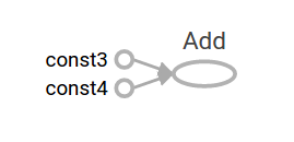
但上面是常量之间的操作,这个总是产生恒定的结果。其实一个图可以接收外部输入的参数,称为 占位符placeholders。这个占位符之后是可以提供值的。如下:其实和之前的实例是一样的:
a = tf.placeholder(tf.float32)
b = tf.placeholder(tf.float32)
adder_node = a + b  # + provides a shortcut for tf.add(a, b)
前面三行有点像一个函数,我们定义了两个输入参数,然后对他们进行操作。我们可以利用feed_dict参数指定的张量,对这些占位符提供具体的值。如下:
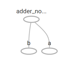
print(sess.run(adder_node, {a: 3, b:4.5}))
print(sess.run(adder_node, {a: [1,3], b: [2, 4]}))
resulting in the output
 7.5
[ 3.  7.]
在tensorboard中,可视化的图如下:
在ML中,我们通常希望一个模型,可以让任意值输入,如上面的一个。为了能让模型得到训练,我们需要能够修改图得到相同的输入新的输出。变量就允许我们添加训练参数图。他们是用类型和初始值构造的:
W = tf.Variable([.3], tf.float32)
b = tf.Variable([-.3], tf.float32)
x = tf.placeholder(tf.float32)
linear_model = W * x + b
常量初始化的时候只要调用tf.constant即可,且他们的值不会发生变化。但是当你调用tf.Variable时,变量并不能初始化。需要明确的调用如下操作:
init = tf.global_variables_initializer()
sess.run(init)
注:有时候,global_variables_initializer()随版本变动,需要注意进行对应更改。 这里的init操作仍然看作是graph的一部分内容。只有真正执行sess.run操作之后才完成初始化操作。
这里的x作为一个占位符,我们可以在评估这个模型的时候同时输入x的多个值,如下:
print(sess.run(linear_model, {x:[1,2,3,4]}))
to produce the output
[ 0. 0.30000001 0.60000002 0.90000004]
现在我们已经建立了一个模型,但我们并不知道他有多好。对其评估的话需要训练数据,我们需要一个Y占位符提供所需的值,而且写一个损失函数。
我们用标准损失,也就是计算差值的平方和。具体如下:
y = tf.placeholder(tf.float32)
squared_deltas = tf.square(linear_model - y)
loss = tf.reduce_sum(squared_deltas)
print(sess.run(loss, {x:[1,2,3,4], y:[0,-1,-2,-3]}))
当然,这里我们也可以通过人工改变w和b的值,来让结果更完美,如w=-1,b=1.一个variable在初始化的时候被初始为某个值,但之后可以通过tf.assign进行修改。如下:
fixW = tf.assign(W, [-1.])
fixb = tf.assign(b, [1.])
sess.run([fixW, fixb])
print(sess.run(loss, {x:[1,2,3,4], y:[0,-1,-2,-3]}))
The final print shows the loss now is zero.
0.0
这里我们通过手动修改得到了perfect的结果,但是ML要求自动找到正确的模型参数。下面我们讲解一下:
tf.train API
tensorflow提供的优化器可以慢慢地改变每个变量从而最小化损失函数。最简单的优化器是梯度下降(GD)。它根据变量的导数大小对每个变量进行修改。在一般情况下,人工求导繁琐且易错,TF只需要tf.gradients这个函数就能自动求解。实例如下:
optimizer = tf.train.GradientDescentOptimizer(0.01)
train = optimizer.minimize(loss)
sess.run(init) # reset values to incorrect defaults.
for i in range(1000):
  sess.run(train, {x:[1,2,3,4], y:[0,-1,-2,-3]})

print(sess.run([W, b]))
results in the final model parameters:
 [array([-0.9999969], dtype=float32), array([ 0.99999082],
 dtype=float32)]
至此,我们已经完成了基本的ML。下面是一些更高层的抽象。代码自己体会。
下面是完成线性回归模型的完整代码:
import numpy as np
import tensorflow as tf

# Model parameters
W = tf.Variable([.3], tf.float32)
b = tf.Variable([-.3], tf.float32)
# Model input and output
x = tf.placeholder(tf.float32)
linear_model = W * x + b
y = tf.placeholder(tf.float32)
# loss
loss = tf.reduce_sum(tf.square(linear_model - y)) # sum of the squares
# optimizer
optimizer = tf.train.GradientDescentOptimizer(0.01)
train = optimizer.minimize(loss)
# training data
x_train = [1,2,3,4]
y_train = [0,-1,-2,-3]
# training loop
init = tf.global_variables_initializer()
sess = tf.Session()
sess.run(init) # reset values to wrong
for i in range(1000):
  sess.run(train, {x:x_train, y:y_train})

# evaluate training accuracy
curr_W, curr_b, curr_loss  = sess.run([W, b, loss], {x:x_train, y:y_train})
print("W: %s b: %s loss: %s"%(curr_W, curr_b, curr_loss))
When run, it produces
W: [-0.9999969] b: [ 0.99999082] loss: 5.69997e-11
This more complicated program can still be visualized in TensorBoard 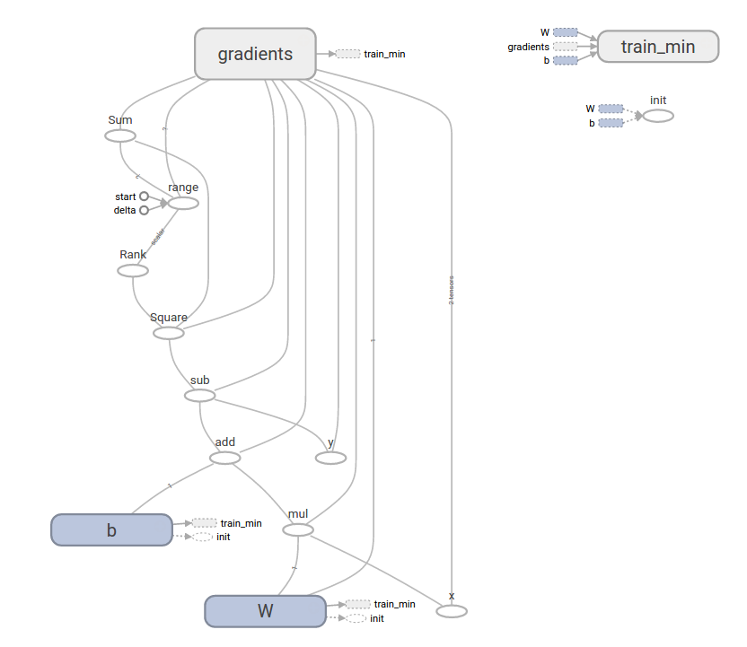
tf.contrib.learn
tf.contrib.learn在训练循环、评估循环、管理数据集和管理feeding方面简化了ML的机制。提供了很多通用模型。
基本的使用:
下面看一下在tf.contrib.learn下面,之前的输入线性回归模型可以如何简化!!!
import tensorflow as tf
# NumPy is often used to load, manipulate and preprocess data.
import numpy as np

# Declare list of features. We only have one real-valued feature. There are many
# other types of columns that are more complicated and useful.
features = [tf.contrib.layers.real_valued_column("x", dimension=1)]

# An estimator is the front end to invoke training (fitting) and evaluation
# (inference). There are many predefined types like linear regression,
# logistic regression, linear classification, logistic classification, and
# many neural network classifiers and regressors. The following code
# provides an estimator that does linear regression.
estimator = tf.contrib.learn.LinearRegressor(feature_columns=features)

# TensorFlow provides many helper methods to read and set up data sets.
# Here we use `numpy_input_fn`. We have to tell the function how many batches
# of data (num_epochs) we want and how big each batch should be.
x = np.array([1., 2., 3., 4.])
y = np.array([0., -1., -2., -3.])
input_fn = tf.contrib.learn.io.numpy_input_fn({"x":x}, y, batch_size=4,
                                              num_epochs=1000)

# We can invoke 1000 training steps by invoking the `fit` method and passing the
# training data set.
estimator.fit(input_fn=input_fn, steps=1000)

# Here we evaluate how well our model did. In a real example, we would want
# to use a separate validation and testing data set to avoid overfitting.
estimator.evaluate(input_fn=input_fn)
When run, it produces
{'global_step': 1000, 'loss': 1.9650059e-11}
A custom model
tf.contrib.learn does not lock you into its predefined models. Suppose we wanted to create a custom model that is not built into TensorFlow. We can still retain the high level abstraction of data set, feeding, training, etc. oftf.contrib.learn. For illustration, we will show how to implement our own equivalent model to LinearRegressorusing our knowledge of the lower level TensorFlow API.
To define a custom model that works with tf.contrib.learn, we need to use tf.contrib.learn.Estimator.tf.contrib.learn.LinearRegressor is actually a sub-class of tf.contrib.learn.Estimator. Instead of sub-classing Estimator, we simply provide Estimator a function model_fn that tells tf.contrib.learn how it can evaluate predictions, training steps, and loss. The code is as follows:
import numpy as np
import tensorflow as tf
# Declare list of features, we only have one real-valued feature
def model(features, labels, mode):
  # Build a linear model and predict values
  W = tf.get_variable("W", [1], dtype=tf.float64)
  b = tf.get_variable("b", [1], dtype=tf.float64)
  y = W*features['x'] + b
  # Loss sub-graph
  loss = tf.reduce_sum(tf.square(y - labels))
  # Training sub-graph
  global_step = tf.train.get_global_step()
  optimizer = tf.train.GradientDescentOptimizer(0.01)
  train = tf.group(optimizer.minimize(loss),
                   tf.assign_add(global_step, 1))
  # ModelFnOps connects subgraphs we built to the
  # appropriate functionality.
  return tf.contrib.learn.ModelFnOps(
      mode=mode, predictions=y,
      loss=loss,
      train_op=train)

estimator = tf.contrib.learn.Estimator(model_fn=model)
# define our data set
x = np.array([1., 2., 3., 4.])
y = np.array([0., -1., -2., -3.])
input_fn = tf.contrib.learn.io.numpy_input_fn({"x": x}, y, 4, num_epochs=1000)

# train
estimator.fit(input_fn=input_fn, steps=1000)
# evaluate our model
print(estimator.evaluate(input_fn=input_fn, steps=10))
When run, it produces
{'loss': 5.9819476e-11, 'global_step': 1000}
Notice how the contents of the custom model() function are very similar to our manual model training loop from the lower level API.