蒙特利尔的麦吉尔大学的计算几何课程资料:
原文链接:http://cgm.cs.mcgill.ca/~godfried/teaching/cg-projects/98/normand/main.html
1. Introduction
When talking about distances, we usually mean the shortest : for instance, if a point X is said to be at distance D of a polygon P, we generally assume that D is the distance from X to the nearest point of P. The same logic applies for polygons : if two polygons A and B are at some distance from each other, we commonly understand that distance as the shortest one between any point of A and any point of B. Formally, this is called a minimin function, because the distance D between A and B is given by :
| |
 |
(eq. 1) |
This equation reads like a computer program : « for every point a of A, find its smallest distance to any point b of B ; finally, keep the smallest distance found among all points a ».
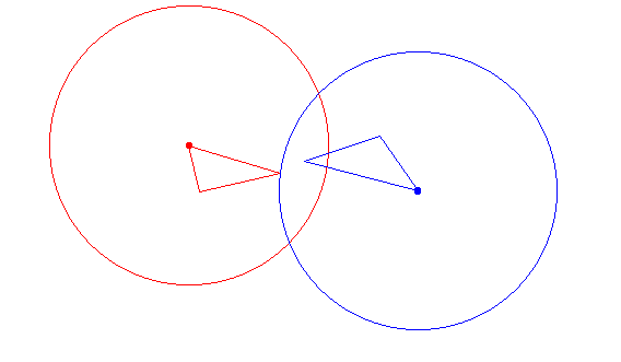
That definition of distance between polygons can become quite unsatisfactory for some applications ; let's see for example fig. 1. We could say the triangles are close to each other considering their shortest distance, shown by their red vertices. However, we would naturally expect that a small distance between these polygons means that no point of one polygon is far from the other polygon. In this sense, the two polygons shown in fig. 1 are not so close, as their furthest points, shown in blue, could actually be very far away from the other polygon. Clearly, the shortest distance is totally independent of each polygonal shape.
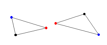
|
Figure 1 : |
The shortest distance doesn't consider the whole shape. |
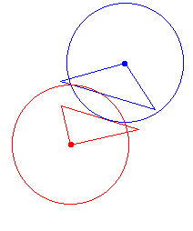
Another example is given by fig. 2, where we have the same two triangles at the same shortest distance than in fig. 1, but in different position. It's quite obvious that the shortest distance concept carries very low informative content, as the distance value did not change from the previous case, while something did change with the objects.
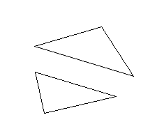
|
Figure 2 : |
The shortest distance doesn't account for the position of the objects. |
As we'll see in the next section, in spite of its apparent complexity, the Hausdorff distance does capture these subtleties, ignored by the shortest distance.
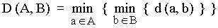
Named after Felix Hausdorff (1868-1942), Hausdorff distance is the « maximum distance of a set to the nearest point in the other set » [Rote91]. More formally, Hausdorff distance from set A to set B is a maximin function, defined as
| |
 |
(eq. 2) |
where a and b are points of sets A and B respectively, and d(a, b) is any metric between these points ; for simplicity, we'll take d(a, b) as the Euclidian distance between a and b. If for instance A and B are two sets of points, a brute force algorithm would be :
Brute force algorithm : 1. h = 0
2. for every point ai of A,
2.1 shortest = Inf ;
2.2 for every point bj of B
dij = d (ai , bj )
if dij < shortest then
shortest = dij
2.3 if shortest > h then
h = shortest
|
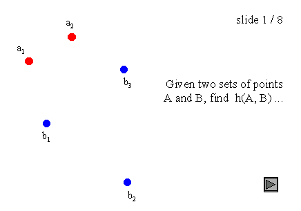 Figure 3 : Hausdorff distance on point sets. |
This is illustrated in fig. 3 : just click on the arrow to see the basic steps of this computation. This algorithm obviously runs in O(n m) time, with n and m the number of points in each set.
It should be noted that Hausdorff distance is oriented (we could say asymmetric as well), which means that most of times h(A, B) is not equal to h(B, A). This general condition also holds for the example of fig. 3, as h(A, B) = d(a1, b1), while h(B, A) = d(b2, a1). This asymmetry is a property of maximin functions, while minimin functions are symmetric.
A more general definition of Hausdorff distance would be :
| |
H (A, B) = max { h (A, B), h (B, A) }
|
(eq. 3) |
which defines the Hausdorff distance between A and B, while eq. 2 applied to Hausdorff distance from A to B (also called directed Hausdorff distance). The two distances h(A, B) and h(B, A) are sometimes termed as forward and backward Hausdorff distances of A to B. Although the terminology is not stable yet among authors, eq. 3 is usually meant when talking about Hausdorff distance. Unless otherwise mentionned, from now on we will also refer to eq. 3 when saying "Hausdorff distance".
If sets A and B are made of lines or polygons instead of single points, then H(A, B) applies to all defining points of these lines or polygons, and not only to their vertices. The brute force algorithm could no longer be used for computing Hausdorff distance between such sets, as they involve an infinite number of points.

So, what about the polygons of fig. 1 ? Remember, some of their points were close, but not all of them. Hausdorff distance gives an interesting measure of their mutual proximity, by indicating the maximal distance between any point of one polygon to the other polygon. Better than the shortest distance, which applied only to one point of each polygon, irrespective of all other points of the polygons.
|
Figure 4 : |
Hausdorff distance shown around extremum of each triangles of fig. 1. Each circle has a radius of H( P1 , P2). |
The other concern was the insensitivity of the shortest distance to the position of the polygons. We saw that this distance doesn't consider at all the disposition of the polygons. Here again, Hausdorff distance has the advantage of being sensitive to position, as shown in fig.5.
|
Figure 5 : |
Hausdorff distance for the triangles of fig. 4 at the same shortest distance, but in different position. |
3.1 Assumptions
Throughout the rest of our discussion, we assume the following facts about polygons A and B :
- Polygons A and B are simple convex polygons ;
- Polygons A and B are disjoint from each other, that is :
- they don't intersect together ;
- no polygon contains the other.
3.2 Lemmas
The algorithm explained in the next section is based on three geometric observations, presented here. In order to simplify the text, we assume two points a and b that belong respectively to polygons A and B, such that :
d (
a,
b) = h (A, B)
In simple words, a is the furthest point of polygon A relative to polygon B, while b is the closest point of polygon B relative to polygon A.
| Lemma 1b : |
The perpendicular to ab at b is a supporting line of B, and a and B are on different sides relative to that line. Proof of lemma 1b |
| Lemma 2 : |
There is a vertex x of A such that the distance from x to B is equal to h (A, B). Proof of lemma 2 |
| Lemma 3 : |
Let bi be the closest point of B from a vertex a i of A. If µ is the moving direction (clockwise or counterclockwise) from bi to bi+1 then, for a complete cycle through all vertices of A, µ changes no more than twice. Proof of lemma 3 |
3.3 Algorithm
The algorithm presented here was proposed by [Atallah83]. Its basic strategy is to compute successively h(A,B) and h(B, A) ; because of lemma 2, there is no need to query every point of the starting polygon, but only its vertices.
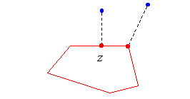
| An important fact used by this algorithm is that a closest point can only be a vertex of the target polygon, or the foot z of a line perpendicular to one of its edges.
This fact suggests a function to check for the existence of a possible closest point. Given a source point a and a target edge defined by a point b1 and a vertex b2 : |
|
Function z = CheckForClosePoint (a, b1 , b2 ) :
Compute the position z where the line that passes through b1 and b2 crosses its perpendicular through a ;
if z is between b1 b2 then return z ;
else compute at b2 a line P perpendicular to the line ab2 ;
if P is a supporting line of B then return b2 ;
else return NULL.
That function obviously uses lemma 1b to decide whether or not the closest point of B might be located on the target edge, that should be close to a. It also supposes that the source point a and b2 are not located on different sides of the perpendicular to [b1b2 ] at b1, accordingly to lemma 3.
Now we are ready for the main algorithm ; the vertices of both polygons are presumed to be enumerated counterclockwise :
|
Algorithm for computing h(A, B) : 1. From a1, find the closest point b1 and compute d1 = d ( a1, b1 )
2. h(A, B) = d1
3. for each vertex ai of A,
3.1 if ai+1 is to the left of aibi
find bi+1 , scanning B counterclockwise with CheckForClosePoint from bi
if ai+1 is to the right of aibi
find bi+1 , scanning B clockwise with CheckForClosePoint from bi
if ai+1 is anywhere on aibi
bi+1 = bi
3.2 Compute di+1 = d (ai+1 , bi+1 )
3.3 h (A, B) = max { h (A, B), di+1 }
|
3.4 Complexity
If polygons A and B respectively have n and m vertices, then :
- Step 1 can clearly be done in O(m) time ;
- Step 2 takes constant time O(1) ;
- Step 3 will be executed (n-1) times, that is O(n) ;
- Step 3.1 will not be executed in total more than O(2m). This is a consequence of lemma 3, which guarantees that polygon B can not be scanned more than twice ;
- Steps 3.2 and 3.3 are done in constant time O(1) ;
So the algorithm for computing h(A, B) takes :
O(m) + O(n) + O(2m) = O(n+m)
To find H(A, B), the algorithm needs to executed twice ; the total complexity for computing Hausdorff distance then stays linear to O(n+m).
3.5 Interactive applet
This applet illustrates the algorithm for computing h(A,B). You only need to draw two polygons, and then press the "step" or "run" button. Left click to define a new vertex, and close the polygon by clicking near the first vertex. Polygon A is the first one you draw, in green, while polygon B appears next, in red.
The algorithm was slightly modified to make it more appealing visually. Even if this algorithm is intended for two polygons totally separated from each other, it also works when B is inside A. However, it won't work if A is inside of B, or when A and B are partially intersecting. You're allowed anyway to try these cases to see what happens !
When defining your polygons, you will see a yellow area that indicates where you can add the next vertex, so the polygon keeps convex. The applet won't let you define a non-convex polygon.
Please notice that the first time you draw the second half of a polygon, you will have to wait a few seconds until the Jama package loads.
import java.awt.*;
import java.applet.Applet;
import java.util.Vector;
import java.lang.Math;
import Jama.*;
public class Hausdorff extends Applet
{
PolyArea area;
Panel control;
Button runStop;
boolean running;
TextField comment;
public void init()
{
setLayout (new BorderLayout());
comment = new TextField ("", 60);
comment.setEditable (false);
area = new PolyArea (comment);
add ("Center", area);
control = new Panel();
control.add (new Button ("step"));
runStop = new Button ("run");
control.add (runStop);
control.add (new Button ("reset"));
control.add (comment);
add("South", control);
running = false;
}
public boolean action (Event evt, Object arg)
{
if ("step".equals(arg))
area.stepAlgo();
if ("run".equals(arg))
{
runStop.setLabel ("stop");
startAnim();
running = true;
}
if ("stop".equals(arg))
{
runStop.setLabel ("run");
stopAnim();
running = false;
}
if ("reset".equals(arg))
{
remove (area);
stopAnim();
area = new PolyArea (comment);
add ("Center", area);
runStop.setLabel ("run");
validate();
stopAnim();
running = false;
}
return true;
}
public void start()
{
if (running)
startAnim();
}
public void stop()
{
stopAnim();
}
public void startAnim()
{
if (area.animator == null)
{
area.animator = new Thread (area);
}
area.animator.start();
}
public void stopAnim()
{
area.animator = null;
}
public void paint(Graphics g) {
Dimension d = getSize();
g.setColor (Color.black);
g.drawRect(0,0, d.width - 1, d.height - 1);
}
/* This is used to leave room to the black box painted in
* the paint() method. If we don't do that, it is overwritten.
*/
public Insets getInsets() {
return new Insets(3,3,3,3);
}
}
//=============================================================================
/*
* The PolyArea class defines an area that will hold our two polygons.
* It will first create them by catching mouse clicks events and adding
* the points to the polygons, and it will then run the algorithm on the
* polygons.
*/
class PolyArea extends Canvas implements Runnable
{
Dimension offDimension;
Image offImage;
Graphics offGraphics;
TextField comment;
public Thread animator;
FConvexPoly poly1, poly2;
int nextStep;
int currentV1;
FPoint bestV1, bestV2, currentV2;
double bestLength;
int currentRegBase;
boolean band;
Polygon currentRegion;
boolean trigo;
public PolyArea (TextField comment)
{
animator = null;
this.comment = comment;
setBackground (Color.white);
poly1 = new FConvexPoly (Color.green);
poly2 = new FConvexPoly (Color.red);
nextStep = -1;
currentV1 = currentRegBase = -1;
bestV1 = bestV2 = currentV2 = null;
band = false;
currentRegion = null;
bestLength = 0;
trigo = true;
comment.setText ("Please enter the first polygon");
comment.setBackground (new Color (220, 255, 230));
comment.setForeground (Color.black);
}
public boolean handleEvent (Event e)
{
switch (e.id)
{
case Event.MOUSE_DOWN:
if (nextStep == -1)
{
if (! poly1.isClosed())
{
poly1.addPoint (new FPoint (e.x, e.y));
if (poly1.isClosed())
{
comment.setText ("Please enter the second polygon");
comment.setBackground (new Color (255, 220, 220));
}
}
else
{
poly2.addPoint (new FPoint (e.x, e.y));
if (poly2.isClosed())
{
comment.setText ("Press step or run to see the algorithm");
comment.setBackground (new Color (255, 255, 220));
nextStep = 0;
}
}
}
repaint();
return true;
default:
return false;
}
}
/* This method performs a step in the algorithm. It is called either
* by the applet when the "step" button is clicked, or by the animator
* thread if this one is running. */
public void stepAlgo ()
{
Point p;
switch (nextStep)
{
case 0:
comment.setText ("Searching for the first vertex");
comment.setBackground (new Color (255, 235, 200));
currentV1 = 0;
currentRegBase = 0;
band = false;
makeRegion();
p = poly1.getPoint (currentV1);
if (currentRegion.inside (p.x, p.y))
nextStep = 2;
else
nextStep = 1;
repaint();
break;
case 1:
if (! band)
band = true;
else
{
currentRegBase++;
band = false;
}
makeRegion();
p = poly1.getPoint (currentV1);
if (currentRegion.inside (p.x, p.y))
nextStep = 2;
else
nextStep = 1;
repaint();
break;
case 2:
comment.setText ("Computing length");
comment.setBackground (new Color (255, 220, 255));
makeV2();
bestV1 = poly1.getFPoint (currentV1);
bestV2 = currentV2;
bestLength = new FVector (bestV1, bestV2).length();
nextStep = 3;
repaint();
break;
case 3:
comment.setText ("Searching for the next vertex");
comment.setBackground (new Color (255, 235, 200));
if (new FVector (currentV2, poly1.getFPoint (currentV1)).isTrigo
(new FVector (currentV2, poly1.getFPoint (currentV1 + 1))))
trigo = true;
else
trigo = false;
currentV1++;
currentV2 = null;
if (poly1.getFPoint (currentV1) == poly1.getFPoint (0))
nextStep = 7;
else
{
p = poly1.getPoint (currentV1);
if (currentRegion.inside (p.x, p.y))
nextStep = 5;
else
nextStep = 4;
}
repaint();
break;
case 4:
if ((trigo || !poly2.isTrigo()) && !(trigo && !poly2.isTrigo()))
if (! band)
band = true;
else
{
currentRegBase++;
band = false;
}
else
if (! band)
{
currentRegBase--;
band = true;
}
else
band = false;
makeRegion();
p = poly1.getPoint (currentV1);
if (currentRegion.inside (p.x, p.y))
nextStep = 5;
else
nextStep = 4;
repaint();
break;
case 5:
comment.setText ("Comparing this length with the previous best");
comment.setBackground (new Color (255, 220, 255));
makeV2();
if (new FVector (poly1.getFPoint (currentV1), currentV2).length() > bestLength)
nextStep = 6;
else
nextStep = 3;
repaint();
break;
case 6:
comment.setText ("This is the new best length");
comment.setBackground (new Color (220, 255, 220));
bestV1 = poly1.getFPoint (currentV1);
bestV2 = currentV2;
bestLength = new FVector (bestV1, bestV2).length();
nextStep = 3;
repaint();
break;
case 7:
comment.setText ("Hausdorff distance from poly 1 to poly 2");
comment.setBackground (new Color (220, 220, 255));
currentV1 = -1;
currentV2 = null;
currentRegion = null;
animator = null;
repaint();
break;
default:
break;
}
}
/* The paint method draws the current state of the algorithm in the
* given Graphics, including the two polygons, the yellow region and
* the important points. */
public void paint (Graphics g)
{
poly1.fill (g);
poly2.fill (g);
if (currentRegion != null)
{
g.setColor (Color.yellow);
g.fillPolygon (currentRegion);
}
poly1.draw (g);
poly2.draw (g);
if (currentV1 >= 0)
{
Point p = poly1.getPoint (currentV1);
g.setColor (Color.blue);
g.drawOval (p.x-5, p.y-5, 10, 10);
}
if (currentV2 != null)
{
Point p1 = poly1.getPoint (currentV1);
Point p2 = currentV2.getPoint();
g.setColor (Color.blue);
g.drawOval (p2.x-5, p2.y-5, 10, 10);
g.setColor (Color.blue);
g.drawLine (p1.x, p1.y, p2.x, p2.y);
}
if (bestV1 != null)
{
Point p1 = bestV1.getPoint();
Point p2 = bestV2.getPoint();
g.setColor (Color.magenta);
g.drawLine (p1.x, p1.y, p2.x, p2.y);
}
}
/* When called by the AWT, the update method clears its offscreen
* buffer, calls paint() to draw in it, and then copies the buffer to the
* screen. */
public void update (Graphics g)
{
Dimension d = size();
if ((offGraphics == null) ||
(d.width != offDimension.width) ||
(d.height != offDimension.height))
{
offDimension = d;
offImage = createImage(d.width, d.height);
offGraphics = offImage.getGraphics();
}
offGraphics.setColor (getBackground());
offGraphics.fillRect (0, 0, d.width, d.height);
paint (offGraphics);
g.drawImage (offImage, 0, 0, this);
}
/* This method is called in the algorithm to make the new
* yellow polygon that corresponds to the sweeping yellow
* region. */
void makeRegion()
{
Polygon region;
FPoint p1, p2;
FVector v1, v2, edge;
p1 = poly2.getFPoint (currentRegBase);
p2 = poly2.getFPoint (currentRegBase + 1);
edge = new FVector (p1, p2);
if (poly2.isTrigo())
v1 = edge.normal().mult(-1);
else
v1 = edge.normal();
if (band)
{
currentRegion = FConvexPoly.infiniteRegion (p1, v1, p2, v1);
}
else
{
p2 = poly2.getFPoint (currentRegBase - 1);
edge = new FVector (p2, p1);
if (poly2.isTrigo())
v2 = edge.normal().mult(-1);
else
v2 = edge.normal();
currentRegion = FConvexPoly.infiniteRegion (p1, v1, p1, v2);
}
}
/* This method creates the new end of the current smallest distance
* that's on the red polygon. If the current vertex of the green polygon
* is in a yellow sector, it corresponds to the current vertex of the red
* polygon. If it is in a band, it is the foot of the perpendicular to the
* current edge of the red polygon that goes through the vertex. */
void makeV2()
{
if (! band)
currentV2 = poly2.getFPoint (currentRegBase);
else
{
FPoint p1, p2;
FVector vBase;
FLine baseLine, perpendicular;
p1 = poly2.getFPoint (currentRegBase);
p2 = poly2.getFPoint (currentRegBase + 1);
vBase = new FVector (p1, p2);
baseLine = new FLine (p1, vBase);
p2 = poly1.getFPoint (currentV1);
perpendicular = new FLine (p2, vBase.normal());
currentV2 = baseLine.intersect (perpendicular);
}
}
/* The run method is called by the virtual machine to perform the
* automated animation of the algorithm. It calls the stepAlgo() method
* three times per second to animate the algorithme. */
public void run()
{
Thread.currentThread().setPriority(Thread.MIN_PRIORITY);
long startTime = System.currentTimeMillis();
while (Thread.currentThread() == animator)
{
stepAlgo();
try
{
startTime += 300;
Thread.sleep (Math.max (0, startTime-System.currentTimeMillis()));
}
catch (InterruptedException e) { break; }
}
}
}
//=============================================================================
/*
* The FConvexPoly class represents a convex polygon.
*/
class FConvexPoly
{
public Vector v;
boolean closed;
boolean trigo;
Color polyColor;
public FConvexPoly (Color c)
{
v = new Vector();
closed = false;
trigo = false;
polyColor = c;
}
public boolean isClosed ()
{
return closed;
}
public boolean isTrigo ()
{
return trigo;
}
public Point getPoint (int i)
{
return ((FPoint) v.elementAt (MesMath.mod (i, v.size()))).getPoint();
}
public FPoint getFPoint (int i)
{
return (FPoint) v.elementAt (MesMath.mod (i, v.size()));
}
public void addPoint (FPoint p)
{
if (! closed)
{
if (v.size() < 3)
{
v.addElement (p);
if (v.size() == 3)
trigo = firstVector().isTrigo (lastVector());
}
else
{
if (p.equals ((FPoint) v.firstElement()))
closed = true;
else
{
if (isNextOK (p))
v.addElement (p);
}
}
}
}
public boolean isNextOK (FPoint p)
{
FVector next;
next = new FVector ((FPoint) v.firstElement(), p);
if (firstVector().isTrigo (next) != trigo)
return false;
next = new FVector ((FPoint) v.lastElement(), p);
if (lastVector().isTrigo (next) != trigo)
return false;
next = new FVector ((FPoint) v.firstElement(), p);
if (boundVector().isTrigo (next) == trigo)
return false;
else
return true;
}
public FVector firstVector()
{
return new FVector ((FPoint) v.elementAt (0),
(FPoint) v.elementAt (1));
}
public FVector lastVector()
{
return new FVector ((FPoint) v.elementAt (v.size()-2),
(FPoint) v.elementAt (v.size()-1));
}
public FVector boundVector()
{
return new FVector ((FPoint) v.elementAt (v.size()-1),
(FPoint) v.elementAt (0));
}
/* Draw the filled polygon on the given graphics. */
public void fill (Graphics g)
{
Polygon p = new Polygon();
Point pt, pt2;
FPoint fpt;
for (int a=0; a<v.size(); a++)
{
pt = ((FPoint) v.elementAt (a)).getPoint();
p.addPoint (pt.x, pt.y);
}
g.setColor (polyColor);
g.fillPolygon (p);
if (!closed && v.size() >= 3)
{
Polygon nextReg = new Polygon();
if (lastVector().isTrigo (firstVector()) == trigo)
{
pt = ((FPoint) v.firstElement()).getPoint();
pt2 = ((FPoint) v.lastElement()).getPoint();
nextReg.addPoint (pt.x, pt.y);
nextReg.addPoint (pt2.x, pt2.y);
FLine l1 = new FLine ((FPoint) v.firstElement(),
firstVector());
FLine l2 = new FLine ((FPoint) v.lastElement(),
lastVector());
fpt = l1.intersect (l2);
pt = fpt.getPoint();
nextReg.addPoint (pt.x, pt.y);
}
else
{
FVector firstInv = firstVector().mult (-1);
nextReg = infiniteRegion ((FPoint) v.firstElement(),
firstInv,
(FPoint) v.lastElement(),
lastVector());
}
g.setColor (Color.yellow);
g.fillPolygon (nextReg);
}
}
/* Draw the outline of the polygon on the given graphics. */
public void draw (Graphics g)
{
Point pt, pt2;
g.setColor (Color.blue);
if (v.size() > 0)
{
pt = pt2 = ((FPoint) v.firstElement()).getPoint();
for (int a=0; a<v.size()-1; a++)
{
pt2 = ((FPoint) v.elementAt (a+1)).getPoint();
g.drawLine (pt.x, pt.y, pt2.x, pt2.y);
pt = pt2;
}
pt = ((FPoint) v.firstElement()).getPoint();
if (closed)
g.drawLine (pt.x, pt.y, pt2.x, pt2.y);
else
{
g.setColor (Color.red);
g.drawOval (pt.x-5, pt.y-5, 10, 10);
}
}
}
/* This method returns a Polygon that will look infinite when
* drawn by the Graphics methods. This should not be in here, it should
* not be a static method, but it worked so I left it this way...*/
public static Polygon infiniteRegion (FPoint p1, FVector v1, FPoint p2, FVector v2)
{
Polygon p = new Polygon();
Point pt;
double length;
FVector middle;
pt = p1.getPoint();
p.addPoint (pt.x, pt.y);
if (! p1.equals (p2))
{
pt = p2.getPoint();
p.addPoint (pt.x, pt.y);
}
length = v2.length();
pt = new Point ((int) (p2.x + (v2.x / length * 2000)),
(int) (p2.y + (v2.y / length * 2000)));
p.addPoint (pt.x, pt.y);
middle = (v1.mult (1/v1.length())).add (v2.mult (1/v2.length()));
length = middle.length();
pt = new Point ((int) (middle.x + (middle.x / length * 2000)),
(int) (middle.y + (middle.y / length * 2000)));
p.addPoint (pt.x, pt.y);
length = v1.length();
pt = new Point ((int) (p1.x + (v1.x / length * 2000)),
(int) (p1.y + (v1.y / length * 2000)));
p.addPoint (pt.x, pt.y);
return p;
}
}
//=============================================================================
/*
* The FPoint class represents a point in the plane.
*/
class FPoint
{
static double EPSILON = 10;
double x;
double y;
public FPoint (double x, double y)
{
this.x = x;
this.y = y;
}
public FPoint (int x, int y)
{
this.x = (double) x;
this.y = (double) y;
}
public FPoint (Point p)
{
this.x = (double) p.x;
this.y = (double) p.y;
}
public boolean equals (FPoint p)
{
if (new FVector (this, p).length() < EPSILON)
return true;
else
return false;
}
public Point getPoint()
{
return new Point ((int) x, (int) y);
}
}
//=============================================================================
/*
* The FVector class provides a basic 2-dimensional vector type,
* along with some uselful methods.
*/
class FVector
{
double x;
double y;
public FVector (double x, double y)
{
this.x = x;
this.y = y;
}
public FVector (FPoint a, FPoint b)
{
x = b.x - a.x;
y = b.y - a.y;
}
/* Returns the dot product of the vector with v. */
public double dot (FVector v)
{
return x * v.x + y * v.y;
}
/* Returns the vector normal to this vector. */
public FVector normal()
{
return new FVector (-y, x);
}
/* Return true if v makes an angle with the vector in the
* trigonometric direction (a left turn). */
public boolean isTrigo (FVector v)
{
if (dot (v.normal()) <= 0)
return true;
else
return false;
}
public double length()
{
return Math.sqrt (x*x + y*y);
}
public FVector add (FVector v)
{
return new FVector (x + v.x, y + v.y);
}
public FVector mult (double a)
{
return new FVector (x*a, y*a);
}
}
//=============================================================================
/*
* The FLine class represents a line. Here, it is only used to call
* its intersect() method to compute the intersection of two lines.
*/
class FLine
{
/* The line is under the form ax+by=c */
double a;
double b;
double c;
/*
* Creates a new FLine that goes through p and is supported
* by v.
*/
public FLine (FPoint p, FVector v)
{
FVector vn = v.normal();
a = vn.x;
b = vn.y;
c = a * p.x + b * p.y;
}
/* Creates a new FLine that goes through both a and b. */
public FLine (FPoint a, FPoint b)
{
this (a, new FVector (a, b));
}
/*
* The methode computes the intersection point of two
* lines. We use the JAMA matrix package (see
* <a href="http://math.nist.gov/javanumerics/jama/">
* http://math.nist.gov/javanumerics/jama/</a>
* for details).
*/
public FPoint intersect (FLine l)
{
double[][] tabA = {{ a, b},
{l.a, l.b}};
Matrix matA = new Matrix (tabA);
double[][] tabB = {{ c},
{l.c}};
Matrix matB = new Matrix (tabB);
double[][] tabX = (matA.solve (matB)).getArray();
return new FPoint (tabX[0][0], tabX[1][0]);
}
}
//=============================================================================
/*
* The MesMath class is an abstract class that is used to perform
* division related operations on integers. I haven't been able to tell
* java that I needed my divisions to be rounded toward minus infinity
* rather than zero, so I've had to do it myself.
*/
abstract class MesMath
{
public static int div (int a, int b)
{
if (a >= 0)
return a / b;
else
return (a - b + 1) / b;
}
public static int mod (int a, int b)
{
return a - div (a, b) * b;
}
}
4. Application examples
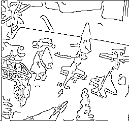
One of the main application of the Hausdorff distance is image matching, used for instance in image analysis, visual navigation of robots, computer-assisted surgery, etc. Basically, the Hausdorff metric will serve to check if a template image is present in a test image ; the lower the distance value, the best the match. That method gives interesting results, even in presence of noise or occlusion (when the target is partially hidden).
Say the small image below is our template, and the large one is the test image :
We want to find if the small image is present, and where, in the large image. The first step is to extract the edges of both images, so to work with binary sets of points, lines or polygons :
Edge extraction is usually done with one of the many edge detectors known in image processing, such as Canny edge detector, Laplacian, Sobel, etc. After applying Rucklidge's algorithm that minimizes Hausdorff distance between two images, the computer found a best match :
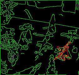
For this example, at least 50 % of the template points had to lie within 1 pixel of a test image point, and vice versa. Some scaling and skew were also allowed, to prevent rejection due to a different viewing angle of the template in the test image (these images and results come from Michael Leventon's pages). Other algorithms might allow more complicated geometric transformations for registering the template on the test image.
In spite of my interest for the topic, an online demo is definitely beyond the scope of this Web project ! So here are some Web resources about image matching with Hausdorff distance :
Glossary
References