机器学习之支持向量机: Support Vector Machines (SVM)
欢迎访问人工智能研究网 课程中心
网址是:http://i.youku.com/studyai

本篇博客介绍机器学习算法之一的支持向量机算法:
- 理解支持向量机(Understanding SVM)
- 使用支持向量机(Using SVM)
- 使用高斯核(Gaussian Kernel)训练SVM分类器
- 使用自定义核(Custom Kernel)训练SVM分类器
- 训练和交叉验证SVM分类器
理解支持向量机(Understanding SVM)
所谓支持向量是指那些在间隔区边缘的训练样本点。 这里的“机(machine,机器)”实际上是一个算法。在机器学习领域,常把一些算法看做是一个机器。支持向量机方法是建立在统计学习理论的VC维理论和结构风险最小原理基础上的,根据有限的样本信息在模型的复杂性(即对特定训练样本的学习精度)和学习能力(即无错误地识别任意样本的能力)之间寻求最佳折中,以求获得最好的推广能力 。 —— [ 百度百科 ]
可分性数据(Separable Data)
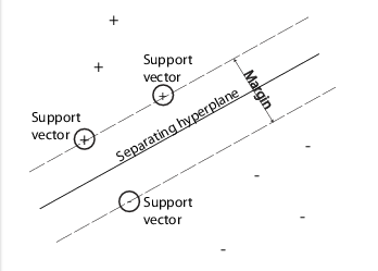
当待分类的数据只有两类时,你就可以用SVM进行分类。SVM通过找到最优超平面对数据进行分类。如果数据是可分的,那么可能有好多个超平面都可以实现分类。但是对SVM来说,最优超平面(best hyper-plane)意味着在两类之间具有最大边际间隔(margin)的那个超平面。”Margin”意味着平行于超平面的没有内部数据点的两个平板(slab)的最大宽度。支持向量(support vectors) 是那些最靠近分离超平面的数据点; 这些点都分布在slab的边界上. 如下图所示:“+”号表示标签为1的样本, and “-”号表示标签为-1的样本
数学表述 原问题:
训练数据是一个
d
维向量集 xi∈Rd 还有与之对应的类别标签集合
yi=±1
. 那么超平面公式可以标示为
<w,x>+b=0
<script type="math/tex; mode=display" id="MathJax-Element-4">
+b=0</script>
其中
w∈Rd
是权值向量,
<w,x>
<script type="math/tex" id="MathJax-Element-6">
</script>是内积,
b
是偏置。
下面的约束优化问题定义了最优分离超平面:
目标函数:minw,b||w||约束条件:yi∗(<w,xi>+b)≥1,i=1,2,⋯,N
支持向量就是那些满足边界条件的数据点
xi
:
yi∗(<w,xi>+b)=1
。
为了数学处理上的方便,上面的目标函数常被替换成等效的形式:
minw,b12<w,w>
, 这是一个带约束的二次规划问题,我们可以用拉格朗日乘数法来求解。我们将正的拉格朗日算子
αi
乘以每一个约束条件,然后从目标函数中减去,如下所示:
Lp=12<w,w>−∑i=1N(αi∗(yi(<w,xi>+b)−1))
为了找到
Lp(w,b)
的驻点,分别对变量
w
和
b求偏导数,并令其等于0,我们可以得到如下的方程组:
w0==∑i=1Nαiyixi∑i=1Nαiyi
得到其最优解
(wˆ,bˆ)
后,对新的样本数据
z
的分类如下进行:
class(z)=sign(wˆ∗z+bˆ)
因为解决二次规划问题的对偶问题要更加简单,所以我们要把原问题重新表述成它的对偶问题。
数学表述 对偶问题:
为了获得对偶问题,我们将上面的方程组代入
Lp
就可以得到对偶问题:
LD=∑i=1Nαi−12∑i=1N∑j=1N(αiαjyiyj<xixj>)
现在,我们只需要在
αi≥0
的范围内最大化目标函数
LD
. 这是一个标准的二次规划问题,我们可以使用Matlab的优化工具箱来求解。一般来说,在
LD
取到最大值时,很多
αi
都等于0了。对偶问题中,非零的
αi
定义了超平面,并且给定了权值向量和偏置正如上面的驻点方程组所表述的那样。与非零的
αi
相对应的数据点
xi
就是支持向量。
在最优解上,
LD
对非零
αi
的微分是等于0的,这导致了
yi(<w,xi>+b)−1=0
。这样我们就可以从此方程中求出偏置
b
了。
不可分性数据(Nonseparable Data)
有些时候,我们的数据无法用一个超平面将其完全严格的分离开来。这时候,SVM通过使用软化边际(soft margin)来构造分离平面,将绝大多数数据点正确的分类。
soft margin有两种标准的形式,都是通过添加松弛变量(lack variables) :si和一个惩罚因子 (penalty factor):
C
.
形式1: L1-norm
目标函数:minw,b,s(12<w,w>+C∑i=1Nsi)约束条件:yi∗(<w,xi>+b)≥1−si,si≥0,i=1,2,⋯,N
形式2:
L2-norm
目标函数:minw,b,s(12<w,w>+C∑i=1Ns2i)约束条件:yi∗(<w,xi>+b)≥1−si,si≥0,i=1,2,⋯,N
上面两种形式的区别在于松弛变量
si
的阶数。Matlab函数
fitsvm 的三个参数选项SMO, ISDA 和L1Qp都是最小化
L1
范数。 在上述两种形式中,我们可以看到增加惩罚因子
C
的值将会在松弛变量上放更大的权重,意味着优化过程将试图达到一个对各类数据的更严格的分离。等效的,减小
C直到0将使得错误分类的重要性下降。
同样的,为了求解带松弛变量的情况,我们将上述形式1中的
L1-norm
约束二次规划问题用拉格朗日乘数法转化为无约束的二次规划问题如下:
Lp(w,b,si,μi)=12<w,w>+C∑iNsi−∑i=1N(αi∗(yi(<w,xi>+b)−(1−si)))−∑iNμisi
其中
μi
是对应于松弛变量
si
的拉格朗日乘子。
对
w,b,si,μi
求偏微分,并且让让梯度等于0,就可以得到驻点方程组,如下:
w0μiαi,===μi,si∑i=1Nαiyixi∑i=1NαiyiC−αi≥0
同样的,我们将上述方程组代入
Lp(w,b,α,μ)
中去,就可以得到其对偶问题的表示:
目标函数:maxαLD=∑i=1Nαi−12∑i=1N∑j=1N(αiαjyiyj<xixj>)约束条件:∑i=1Nαiyi=0and0≤αi≤C
与无松弛变量的对偶问题对比,我们发现上述对偶问题中没有松弛变量
si
和其对应的拉格朗日乘子
μi
,目标函数是完全一样的. 约束条件中的不等式
0≤αi≤C
比无松弛变量的情况多了一个上界
C
,此上界经常被称为盒式约束(box constraint),
C 使得拉格朗日乘子的允许值在一个有界的区域内。
L2-norm
的情况与此非常类似,不再赘述。
Matlab中fitcsvm的实现
为了解决上述的二次规划问题:dual soft-margin problems,Matlab的fitcsvm函数为我们提供了若干不同的算法:
1. 对于one-class或二类分类问题,如果你没有指定训练数据中的期望外点(使用name-value参数:OutlierFraction),那么默认使用Sequential Minimal Optimization (SMO)来求解。SMO求解
L1-norm
对偶问题通过一些列两点最小化。在优化过程中,SMO遵守线性约束
∑iαiyi=0
,而且在模型中显示的包含了偏置项。
2. 对于二类分类问题,如果你指定了训练数据中的期望外点(通过使用name-value参数:OutlierFraction来指定),那么默认使用Iterative Single Data Algorithm (ISDA)来求解。与SMO相同的是,ISDA也最小化
L1-norm
对偶问题。不同的是,ISDA最小化目标函数通过一系列单点最小化。在优化过程中,ISDA不遵守线性约束
∑iαiyi=0
,而且在模型中也不包含偏置项。
3. For one-class or binary classification, and if you have an Optimization Toolbox license, you can choose to use quadprog to solve the one-norm problem. quadprog uses a good deal of memory, but solves quadratic programs to a high degree of precision .
在一些二类分类问题中,无法使用一个简单的超平面作为分割标准。为了解决这样的问题,我们采用一种基于再生核理论(the theory of reproducing kernels)的数学方法,该方法非常好的保持了SVM的简洁易用的特点。
1. 有一类函数
K(x,y)
具有下列的一些性质:存在一个线性空间
S
以及一个将x映射到
S
的映射φ:
K(x,y)=<φ(x),φ(y)>
; 其中内积运算发生在线性空间
S
.
2. 这类函数包括以下几个:
a. 多项式函数(Polynomials):
对某些正整数d,
K(x,y)=(1+<x,y>)d
b.高斯放射基函数(Radial basis function (Gaussian)):
对某些正整数
σ
,
K(x,y)=exp(–<(x–y),(x–y)>2σ2)
c.神经网络多层感知器(Multilayer perceptron):
对一个正数
P1
和一个负数
P2
,
K(x,y)=tanh(p1<x,y>+p2).
使用支持向量机(Using SVM)
对于任何的监督学习模型, 我们要先训练一个SVM分类器,然后再交叉验证之,最后在用训练好的机器去预测或分类新的数据. 特别值得一提的是,为了获得比较满意的预测精度, 你可以尝试各种各样的核函数, 并且要细心的调教核函数的参数.
训练一个 SVM 分类器
训练一个SVM分类器模型的最通用语法如下:
SVMModel = fitcsvm(X,Y,'KernelFunction','rbf','Standardize',true,'ClassNames',{'negClass','posClass'});
输入参数如下:
1. X — Matrix of predictor data, 其中每一行是一个样本特征向量, 每一列是一个 predictor.
2. Y — Array of class label,其中每一行与X矩阵的对应行关联.
3. KernelFunction — 对两类分类问题,默认值是线性核 ‘linear’ , 使用一个超平面分离数据. The value ‘rbf’ is the default for one-class learning, and uses a Gaussian radial basis function. An important step to successfully train an SVM classifier is to choose an appropriate kernel function.
4. Standardize — Flag indicating whether the software should standardize the predictors before training the classifier.
5. ClassNames — Distinguishes between the negative and positive classes, or specifies which classes to include in the data. The negative class is the first element (or row of a character array), e.g., ‘negClass’, and the positive class is the second element (or row of a character array), e.g., ‘posClass’. ClassNames must be the same data type as Y. It is good practice to specify the class names, especially if you are comparing the performance of different classifiers.
The resulting, trained model (SVMModel) contains the optimized parameters from the SVM algorithm, enabling you to classify new data.
使用训好的 SVM 分类新数据
Classify new data using predict. The syntax for classifying new data using a trained SVM classifier (SVMModel) is:
[label,score] = predict(SVMModel,newX);
The resulting vector, label, represents the classification of each row in X. score is an n-by-2 matrix of soft scores. Each row corresponds to a row in X, which is a new observation. The first column contains the scores for the observations being classified in the negative class, and the second column contains the scores observations being classified in the positive class.
To estimate posterior probabilities rather than scores, first pass the trained SVM classifier (SVMModel) to fitPosterior, which fits a score-to-posterior-probability transformation function to the scores. The syntax is:
ScoreSVMModel = fitPosterior(SVMModel,X,Y);
The property ScoreTransform of the classifier ScoreSVMModel contains the optimal transformation function. Pass ScoreSVMModel to predict. Rather than returning the scores, the output argument score contains the posterior probabilities of an observation being classified in the negative (column 1 of score) or positive (column 2 of score) class.
调节一个训好的 SVM 分类器
Try tuning parameters of your classifier according to this scheme:
- Pass the data to fitcsvm, and set the name-value pair arguments ‘KernelScale’,’auto’. Suppose that the trained SVM model is called SVMModel. The software uses a heuristic procedure to select the kernel scale. The heuristic procedure uses subsampling. Therefore, to reproduce results, set a random number seed using rng before training the classifier.
- Cross validate the classifier by passing it to crossval. By default, the software conducts 10-fold cross validation.
Pass the cross-validated SVM model to kFoldLoss to estimate and retain the classification error.
- Retrain the SVM classifier, but adjust the ‘KernelScale’ and ‘BoxConstraint’ name-value pair arguments.
a. BoxConstraint — One strategy is to try a geometric sequence of the box constraint parameter. For example, take 11 values, from 1e-5 to 1e5 by a factor of 10. Increasing BoxConstraint might decrease the number of support vectors, but also might increase training time.
b. KernelScale — One strategy is to try a geometric sequence of the RBF sigma parameter scaled at the original kernel scale. Do this by:
b1: Retrieving the original kernel scale, e.g., ks, using dot notation: ks = SVMModel.KernelParameters.Scale.
b2: Use as new kernel scales factors of the original. For example, multiply ks by the 11 values 1e-5 to 1e5, increasing by a factor of 10.
Choose the model that yields the lowest classification error.
You might want to further refine your parameters to obtain better accuracy. Start with your initial parameters and perform another cross-validation step, this time using a factor of 1.2. Alternatively, optimize your parameters with fminsearch, as shown in Train and Cross Validate SVM Classifiers.
使用高斯核(Gaussian Kernel)训练SVM分类器
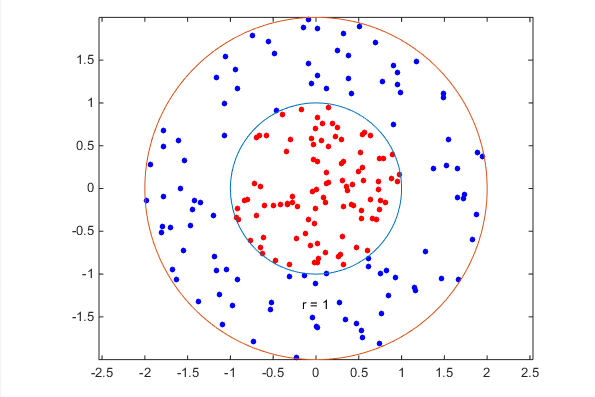
This example shows how to generate a nonlinear classifier with Gaussian kernel function. First, generate one class of points inside the unit disk in two dimensions, and another class of points in the annulus from radius 1 to radius 2. Then, generates a classifier based on the data with the Gaussian radial basis function kernel. The default linear classifier is obviously unsuitable for this problem, since the model is circularly symmetric. Set the box constraint parameter to Inf to make a strict classification, meaning no misclassified training points. Other kernel functions might not work with this strict box constraint, since they might be unable to provide a strict classification. Even though the rbf classifier can separate the classes, the result can be over trained.
Generate 100 points uniformly distributed in the unit disk. To do so, generate a radius
r
as the square root of a uniform random variable, generate an angle t uniformly in
(0,2π)
, and put the point at
(rcos(t),rsin(t))
.
rng(1); % For reproducibility
r = sqrt(rand(100,1)); % Radius
t = 2*pi*rand(100,1);  % Angle
data1 = [r.*cos(t), r.*sin(t)]; % Points
Generate 100 points uniformly distributed in the annulus. The radius is again proportional to a square root, this time a square root of the uniform distribution from 1 through 4.
r2 = sqrt(3*rand(100,1)+1); % Radius
t2 = 2*pi*rand(100,1);      % Angle
data2 = [r2.*cos(t2), r2.*sin(t2)]; % points
Plot the points, and plot circles of radii 1 and 2 for comparison.
figure;
plot(data1(:,1),data1(:,2),'r.','MarkerSize',15)
hold on
plot(data2(:,1),data2(:,2),'b.','MarkerSize',15)
ezpolar(@(x)1);ezpolar(@(x)2);
axis equal
hold off
Put the data in one matrix, and make a vector of classifications.
data3 = [data1;data2];
theclass = ones(200,1);
theclass(1:100) = -1;
Train an SVM classifier with KernelFunction set to ‘rbf’ and BoxConstraint set to Inf. Plot the decision boundary and flag the support vectors.
%Train the SVM Classifier
cl = fitcsvm(data3,theclass,'KernelFunction','rbf',...
    'BoxConstraint',Inf,'ClassNames',[-1,1]);

% Predict scores over the grid
d = 0.02;
[x1Grid,x2Grid] = meshgrid(min(data3(:,1)):d:max(data3(:,1)),...
    min(data3(:,2)):d:max(data3(:,2)));
xGrid = [x1Grid(:),x2Grid(:)];
[~,scores] = predict(cl,xGrid);

% Plot the data and the decision boundary
figure;
h(1:2) = gscatter(data3(:,1),data3(:,2),theclass,'rb','.');
hold on
ezpolar(@(x)1);
h(3) = plot(data3(cl.IsSupportVector,1),data3(cl.IsSupportVector,2),'ko');
contour(x1Grid,x2Grid,reshape(scores(:,2),size(x1Grid)),[0 0],'k');
legend(h,{'-1','+1','Support Vectors'});
axis equal
hold off
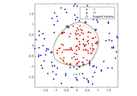
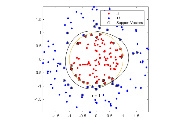
fitcsvm generates a classifier that is close to a circle of radius 1. The difference is due to the random training data.
Training with the default parameters makes a more nearly circular classification boundary, but one that misclassifies some training data. Also, the default value of BoxConstraint is 1, and, therefore, there are more support vectors.
cl2 = fitcsvm(data3,theclass,'KernelFunction','rbf');
[~,scores2] = predict(cl2,xGrid);

figure;
h(1:2) = gscatter(data3(:,1),data3(:,2),theclass,'rb','.');
hold on
ezpolar(@(x)1);
h(3) = plot(data3(cl2.IsSupportVector,1),data3(cl2.IsSupportVector,2),'ko');
contour(x1Grid,x2Grid,reshape(scores2(:,2),size(x1Grid)),[0 0],'k');
legend(h,{'-1','+1','Support Vectors'});
axis equal
hold off
使用自定义核(Custom Kernel)训练SVM分类器
This example shows how to use a custom kernel function, such as the sigmoid kernel, to train SVM classifiers, and adjust custom kernel function parameters.
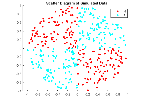
Generate a random set of points within the unit circle. Label points in the first and third quadrants as belonging to the positive class, and those in the second and fourth quadrants in the negative class.
rng(1);  % For reproducibility
n = 100; % Number of points per quadrant

r1 = sqrt(rand(2*n,1));                     % Random radii
t1 = [pi/2*rand(n,1); (pi/2*rand(n,1)+pi)]; % Random angles for Q1 and Q3
X1 = [r1.*cos(t1) r1.*sin(t1)];             % Polar-to-Cartesian conversion

r2 = sqrt(rand(2*n,1));
t2 = [pi/2*rand(n,1)+pi/2; (pi/2*rand(n,1)-pi/2)]; % Random angles for Q2 and Q4
X2 = [r2.*cos(t2) r2.*sin(t2)];

X = [X1; X2];        % Predictors
Y = ones(4*n,1);
Y(2*n + 1:end) = -1; % Labels

%plot the data
figure;
gscatter(X(:,1),X(:,2),Y);
title('Scatter Diagram of Simulated Data')
Create the function mysigmoid.m, which accepts two matrices in the feature space as inputs, and transforms them into a Gram matrix using the sigmoid kernel.
function G = mysigmoid(U,V)
% Sigmoid kernel function with slope gamma and intercept c
gamma = 1;
c = -1;
G = tanh(gamma*U*V' + c);
end
Train an SVM classifier using the sigmoid kernel function. It is good practice to standardize the data.
SVMModel1 = fitcsvm(X,Y,'KernelFunction','mysigmoid','Standardize',true);
SVMModel is a ClassificationSVM classifier containing the estimated parameters.
Plot the data, and identify the support vectors and the decision boundary.
% Compute the scores over a grid
d = 0.02; % Step size of the grid
[x1Grid,x2Grid] = meshgrid(min(X(:,1)):d:max(X(:,1)),...
    min(X(:,2)):d:max(X(:,2)));
xGrid = [x1Grid(:),x2Grid(:)];        % The grid
[~,scores1] = predict(SVMModel1,xGrid); % The scores

figure;
h(1:2) = gscatter(X(:,1),X(:,2),Y);
hold on
h(3) = plot(X(SVMModel1.IsSupportVector,1),...
    X(SVMModel1.IsSupportVector,2),'ko','MarkerSize',10);
    % Support vectors
contour(x1Grid,x2Grid,reshape(scores1(:,2),size(x1Grid)),[0 0],'k');
    % Decision boundary
title('Scatter Diagram with the Decision Boundary')
legend({'-1','1','Support Vectors'},'Location','Best');
hold off
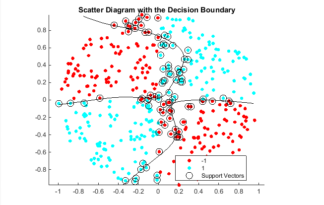
You can adjust the kernel parameters in an attempt to improve the shape of the decision boundary. This might also decrease the within-sample misclassification rate, but, you should first determine the out-of-sample misclassification rate.
Determine the out-of-sample misclassification rate by using 10-fold cross validation.
CVSVMModel1 = crossval(SVMModel1);
misclass1 = kfoldLoss(CVSVMModel1);
misclass1
misclass1 =
0.1350
The out-of-sample misclassification rate is 13.5%.
Set gamma = 0.5; within mysigmoid.m. Then, train an SVM classifier using the adjusted sigmoid kernel. Plot the data and the decision region, and determine the out-of-sample misclassification rate.
SVMModel2 = fitcsvm(X,Y,'KernelFunction','mysigmoid','Standardize',true);
[~,scores2] = predict(SVMModel2,xGrid);

figure;
h(1:2) = gscatter(X(:,1),X(:,2),Y);
hold on
h(3) = plot(X(SVMModel2.IsSupportVector,1),...
    X(SVMModel2.IsSupportVector,2),'ko','MarkerSize',10);
title('Scatter Diagram with the Decision Boundary')
contour(x1Grid,x2Grid,reshape(scores2(:,2),size(x1Grid)),[0 0],'k');
legend({'-1','1','Support Vectors'},'Location','Best');
hold off

CVSVMModel2 = crossval(SVMModel2);
misclass2 = kfoldLoss(CVSVMModel2);
misclass2
misclass2 =
0.0450
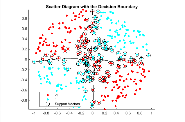
After the sigmoid slope adjustment, the new decision boundary seems to provide a better within-sample fit, and the cross-validation rate contracts by more than 66%.
交叉验证训练SVM分类器
This example classifies points from a Gaussian mixture model. It begins with generating 10 base points for a “green” class, distributed as 2-D independent normals with mean (1,0) and unit variance. It also generates 10 base points for a “red” class, distributed as 2-D independent normals with mean (0,1) and unit variance. For each class (green and red), generate 100 random points as follows:
1. Choose a base point m of the appropriate color uniformly at random.
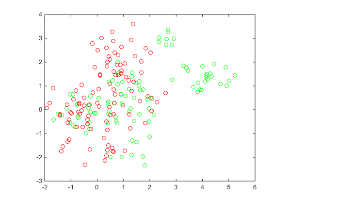
2. Generate an independent random point with 2-D normal distribution with mean m and variance I/5, where I is the 2-by-2 identity matrix.
After generating 100 green and 100 red points, classify them using fitcsvm, and tune the classification using cross validation.
To generate the points and classifier:
Generate the 10 base points for each class.
rng('default')
grnpop = mvnrnd([1,0],eye(2),10);
redpop = mvnrnd([0,1],eye(2),10);

plot(grnpop(:,1),grnpop(:,2),'go')
hold on
plot(redpop(:,1),redpop(:,2),'ro')
hold off
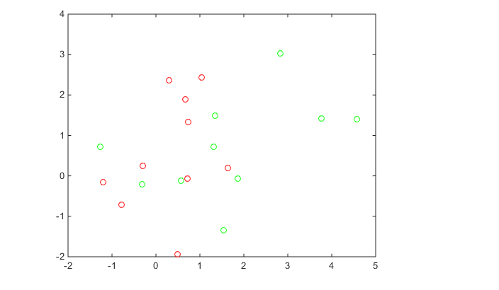
Since many red base points are close to green base points, it is difficult to classify the data points.
Generate the 100 data points of each class:
redpts = zeros(100,2);grnpts = redpts;
for i = 1:100
    grnpts(i,:) = mvnrnd(grnpop(randi(10),:),eye(2)*0.2);
    redpts(i,:) = mvnrnd(redpop(randi(10),:),eye(2)*0.2);
end
figure
plot(grnpts(:,1),grnpts(:,2),'go')
hold on
plot(redpts(:,1),redpts(:,2),'ro')
hold off
Put the data into one matrix, and make a vector grp that labels the class of each point:
cdata = [grnpts;redpts];
grp = ones(200,1);
% Green label 1, red label -1
grp(101:200) = -1;
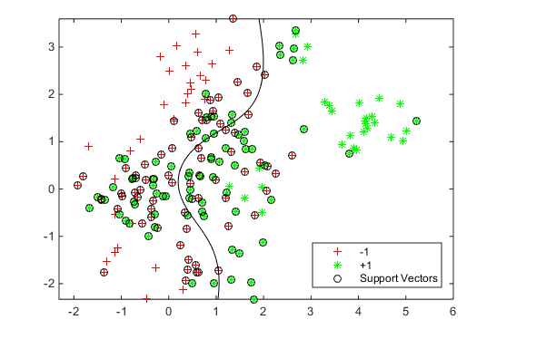
Check the basic classification of all the data using the default parameters:
% Train the classifier
SVMModel = fitcsvm(cdata,grp,'KernelFunction','rbf','ClassNames',[-1 1]);

% Predict scores over the grid
d = 0.02;
[x1Grid,x2Grid] = meshgrid(min(cdata(:,1)):d:max(cdata(:,1)),...
    min(cdata(:,2)):d:max(cdata(:,2)));
xGrid = [x1Grid(:),x2Grid(:)];
[~,scores] = predict(SVMModel,xGrid);

% Plot the data and the decision boundary
figure;
h(1:2) = gscatter(cdata(:,1),cdata(:,2),grp,'rg','+*');
hold on
h(3) = plot(cdata(SVMModel.IsSupportVector,1),...
    cdata(SVMModel.IsSupportVector,2),'ko');
contour(x1Grid,x2Grid,reshape(scores(:,2),size(x1Grid)),[0 0],'k');
legend(h,{'-1','+1','Support Vectors'},'Location','Southeast');
axis equal
hold off

Set up a partition for cross validation. This step causes the cross validation to be fixed. Without this step, the cross validation is random, so a minimization procedure can find a spurious local minimum.
c = cvpartition(200,'KFold',10);
Set up a function that takes an input z=[rbf_sigma,boxconstraint], and returns the cross-validation value of exp(z). The reason to take exp(z) is twofold:
1. rbf_sigma and boxconstraint must be positive.
2. You should look at points spaced approximately exponentially apart.
This function handle computes the cross validation at parameters exp([rbf_sigma,boxconstraint]):
minfn = @(z)kfoldLoss(fitcsvm(cdata,grp,'CVPartition',c,...
    'KernelFunction','rbf','BoxConstraint',exp(z(2)),...
    'KernelScale',exp(z(1))));
Search for the best parameters [rbf_sigma,boxconstraint] with fminsearch, setting looser tolerances than the defaults.
Note that if you have a Global Optimization Toolbox™ license, use patternsearch for faster, more reliable minimization. Give bounds on the components of z to keep the optimization in a sensible region, such as [-5,5], and give a relatively loose TolMesh tolerance.
opts = optimset('TolX',5e-4,'TolFun',5e-4);
[searchmin fval] = fminsearch(minfn,randn(2,1),opts)
searchmin =
1.0246 -0.1569
fval =
0.3100
The best parameters [rbf_sigma;boxconstraint] in this run are:
z = exp(searchmin)
z =
2.7861 0.8548
The surface seems to have many local minima. Try a set of 20 random, initial values, and choose the set corresponding to the lowest fval.
m = 20;
fval = zeros(m,1);
z = zeros(m,2);
for j = 1:m;
    [searchmin fval(j)] = fminsearch(minfn,randn(2,1),opts);
    z(j,:) = exp(searchmin);
end

z = z(fval == min(fval),:)
z =
1.9301 0.7507
Use the z parameters to train a new SVM classifier:
SVMModel = fitcsvm(cdata,grp,'KernelFunction','rbf',...
    'KernelScale',z(1),'BoxConstraint',z(2));
[~,scores] = predict(SVMModel,xGrid);

h = nan(3,1); % Preallocation
figure;
h(1:2) = gscatter(cdata(:,1),cdata(:,2),grp,'rg','+*');
hold on
h(3) = plot(cdata(SVMModel.IsSupportVector,1),...
    cdata(SVMModel.IsSupportVector,2),'ko');
contour(x1Grid,x2Grid,reshape(scores(:,2),size(x1Grid)),[0 0],'k');
legend(h,{'-1','+1','Support Vectors'},'Location','Southeast');
axis equal
hold off
Generate and classify some new data points:
grnobj = gmdistribution(grnpop,.2*eye(2));
redobj = gmdistribution(redpop,.2*eye(2));
newData = random(grnobj,10);
newData = [newData;random(redobj,10)];
grpData = ones(20,1);
grpData(11:20) = -1; % red = -1
v = predict(SVMModel,newData);
g = nan(7,1);
figure;
h(1:2) = gscatter(cdata(:,1),cdata(:,2),grp,'rg','+*');
hold on
h(3:4) = gscatter(newData(:,1),newData(:,2),v,'mc','**');
h(5) = plot(cdata(SVMModel.IsSupportVector,1),...
cdata(SVMModel.IsSupportVector,2),'ko');
contour(x1Grid,x2Grid,reshape(scores(:,2),size(x1Grid)),[0 0],'k');
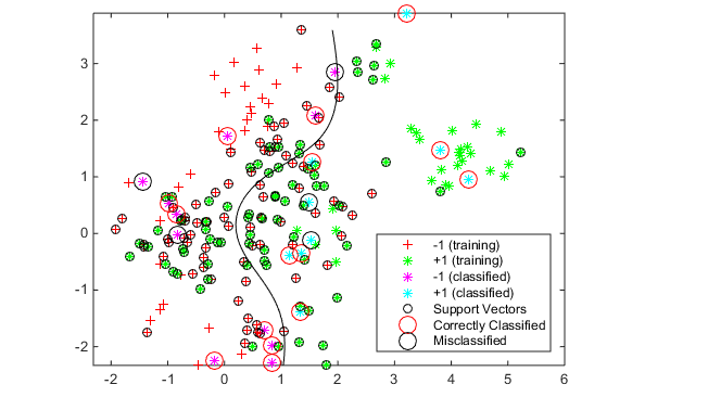
legend(h(1:5),{'-1 (training)','+1 (training)','-1 (classified)',...
'+1 (classified)','Support Vectors'},'Location','Southeast');
axis equal
hold off

See which new data points are correctly classified. Circle the correctly classified points in red, and the incorrectly classified points in black.
mydiff = (v == grpData); % Classified correctly
hold on
for ii = mydiff % Plot red circles around correct pts
    h(6) = plot(newData(ii,1),newData(ii,2),'ro','MarkerSize',12);
end

for ii = not(mydiff) % Plot black circles around incorrect pts
    h(7) = plot(newData(ii,1),newData(ii,2),'ko','MarkerSize',12);
end
legend(h,{'-1 (training)','+1 (training)','-1 (classified)',...
    '+1 (classified)','Support Vectors','Correctly Classified',...
    'Misclassified'},'Location','Southeast');
hold off