cp15_Classifying Images with Deep Convolutional NN_Loss_Cross Entropy_ax.text_mnist_ CelebA_Colab_ck
https://blog.csdn.net/Linli522362242/article/details/108414534
Although IBM’s Deep Blue supercomputer beat the chess world champion Garry Kasparov back in 1996, it wasn’t until fairly recently that computers were able to reliably perform seemingly trivial tasks such as detecting a puppy in a picture or recognizing spoken words. Why are these tasks so effortless to us humans? The answer lies in the fact that perception largely takes place outside the realm of our consciousness, within specialized visual, auditory, and other sensory modules in our brains. By the time sensory information reaches our consciousness, it is already adorned装饰 with high-level features; for example, when you look at a picture of a cute puppy, you cannot choose not to see the puppy, not to notice its cuteness. Nor can you explain how you recognize a cute puppy; it’s just obvious to you. Thus, we cannot trust our subjective experience: perception is not trivial at all, and to understand it we must look at how the sensory modules work.
Convolutional neural networks (CNNs) emerged from the study of the brain’s visual cortex皮层, and they have been used in image recognition since the 1980s. In the last few years, thanks to the increase in computational power, the amount of available training data, and the tricks presented in Chapter 11 for training deep nets, CNNs have managed to achieve superhuman performance on some complex visual tasks. They power image search services, self-driving cars, automatic video classification systems, and more. Moreover, CNNs are not restricted to visual perception: they are also successful at many other tasks, such as voice recognition and natural language processing. However, we will focus on visual applications for now.
In this chapter we will explore where CNNs came from, what their building blocks look like, and how to implement them using TensorFlow and Keras. Then we will discuss some of the best CNN architectures, as well as other visual tasks, including object detection (classifying multiple objects in an image and placing bounding boxes around them) and semantic segmentation (classifying each pixel according to the class of the object it belongs to).
The Architecture of the Visual Cortex
David H. Hubel and Torsten Wiesel performed a series of experiments on cats in 1958 and 1959 (and a few years later on monkeys), giving crucial insights into the structure of the visual cortex (the authors received the Nobel Prize in Physiology or Medicine in 1981 for their work). In particular, they showed that many neurons in the visual cortex have a small local receptive field, meaning they react only to visual stimuli刺激 located in a limited region of the visual field (see Figure 14-1, in which the local receptive fields感官领域 of five neurons are represented by dashed circles). The receptive fields of different neurons may overlap, and together they tile平铺 the whole visual field.

Figure 14-1. Biological neurons in the visual cortex respond to specific patterns in small regions of the visual field called receptive fields; as the visual signal makes its way through consecutive brain modules, neurons respond to more complex patterns in larger receptive fields.
These studies of the visual cortex inspired the neocognitron[niɒ'kɒɡnɪtrɒn]新认知机, introduced in 1980, which gradually evolved into what we now call convolutional neural networks. An important milestone was a 1998 paper by Yann LeCun et al. that introduced the famous LeNet-5 architecture, widely used by banks to recognize handwritten check numbers. This architecture has some building blocks that you already know, such as fully connected layers and sigmoid activation functions, but it also introduces two new building blocks: convolutional layers and pooling layers. Let’s look at them now.
Why not simply use a deep neural network with fully connected layers for image recognition tasks? Unfortunately, although this works fine for small images (e.g., MNIST), it breaks down for larger images because of the huge number of parameters it requires. For example, a 100 × 100–pixel image has 10,000 pixels, and if the first layer has just 1,000 neurons (which already severely restricts the amount of information transmitted to the next layer), this means a total of 10 million connections. And that’s just the first layer. CNNs solve this problem using partially connected layers and weight sharing.
Convolutional Layers


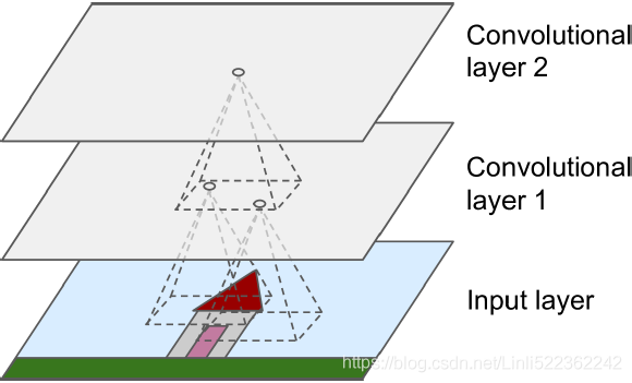 Figure 14-2. CNN layers with rectangular local receptive fields
The most important building block of a CNN is the convolutional layer: neurons in the first convolutional layer (Convolutional layer 1) are not connected to every single pixel in the input image(Input layer) (like they were in the layers discussed in previous chapters), but only to pixels in their receptive fields ( in Input layer)(see Figure 14-2). In turn, each neuron in the second convolutional layer is connected only to neurons located within a small rectangle in the first layer. This architecture allows the network to concentrate on small low-level features in the first hidden layer, then assemble them into larger higher-level features in the next hidden layer, and so on. This hierarchical structure is common in real-world images, which is one of the reasons why CNNs work so well for image recognition.
All the multilayer neural networks we’ve looked at so far had layers composed of a long line of neurons, and we had to flatten input images to 1D before feeding them to the neural network. In a CNN each layer is represented in 2D, which makes it easier to match neurons with their corresponding inputs.
 Figure 14-3. Connections between layers and zero padding
(row: 0 x coumn: 0) <== (row: 0=0, 0+3-1=2 x column: 0=0, 0+3-1=2 )
(row: 1 x coumn: 0) <== (row: 1=1, 1+3-1=3 x column: 0=0, 0+3-1=2 )
A neuron located in row i, column j of a given layer is connected to the outputs of the neurons in the previous layer located in rows i to  , columns j to
  , where
  and
and  are the height and width of the receptive field (see Figure 14-3). In order for a layer to have the same height and width as the previous layer, it is common to add zeros around the inputs, as shown in the diagram. This is called zero padding.
 Figure 14-4. Reducing dimensionality using a stride of 2
(row: 0 x coumn: 0) <== (row: 0*2=0, 0*2+3-1=2 x column: 0*2=0, 0*2+3-1=2 )
(row: 1 x coumn: 0) <== (row: 1*2=2, 1*2+3-1=4 x column: 0*2=0, 0*2+3-1=2 )
It is also possible to connect a large input layer to a much smaller layer by spacing out隔开 the receptive fields, as shown in Figure 14-4. This dramatically reduces the model’s computational complexity. The shift from one receptive field(e.g. 3 × 3 receptive fields) to the next(e.g. 3 × 3 receptive fields) is called the stride步幅,迈. In the diagram, a 5 × 7 input layer (plus zero padding) is connected to a 3 × 4 layer, using 3 × 3 receptive fields and a stride of 2 (in this example the stride is the same in both directions, but it does not have to be so). A neuron located in row i, column j in the upper layer is connected to the outputs of the neurons in the previous layer located in rows  to
to  , columns
  to
to  , where
  and
and  are the vertical and horizontal strides.
Filters
 Figure 14-5. Applying two different filters to get two feature maps
A neuron’s weights can be represented as a small image the size of the receptive field. For example, Figure 14-5 shows two possible sets of weights, called filters (or convolution kernels). The first one is represented as a black square with a vertical white line in the middle (it is a 7 × 7 matrix full of 0s except for the central column, which is full of 1s); neurons using these weights will ignore everything in their receptive field except for the central vertical line (since all inputs will get multiplied by 0, except for the ones located in the central vertical line). The second filter is a black square with a horizontal white line in the middle. Once again, neurons using these weights will ignore everything in their receptive field except for the central horizontal line.
Now if all neurons in a layer use the same vertical line filter (and the same bias term), and you feed the network the input image shown in Figure 14-5 (the bottom image), the layer will output the top-left image. Notice that the vertical white lines get enhanced while the rest gets blurred变得模糊. Similarly, the upper-right image is what you get if all neurons use the same horizontal line filter; notice that the horizontal white lines get enhanced while the rest is blurred out模糊了. Thus, a layer full of neurons using the same filter outputs a feature map, which highlights the areas in an image that activate the filter the most. Of course, you do not have to define the filters manually: instead, during training the convolutional layer will automatically learn the most useful filters for its task, and the layers above will learn to combine them into more complex patterns.
Stacking Multiple Feature Maps
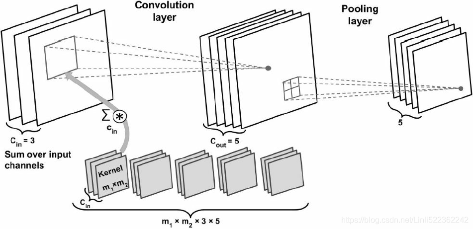
 Figure 14-6. Convolutional layers with multiple feature maps, and images with three color channels
Up to now, for simplicity, I have represented the output of each convolutional layer as a 2D layer, but in reality a convolutional layer has multiple filters(or convolution kernels) (you decide how many) and outputs one feature map per filter, so it is more accurately represented in 3D (see Figure 14-6). It has one neuron per pixel in each feature map, and all neurons within a given feature map share the same parameters (i.e., the same weights and bias term). Neurons in different feature maps use different parameters. A neuron’s receptive field is the same as described earlier, but it extends across all the previous layers’ feature maps. In short, a convolutional layer simultaneously applies multiple trainable filters to its inputs, making it capable of detecting multiple features anywhere in its inputs.
The fact that all neurons in a feature map share the same parameters dramatically reduces the number of parameters in the model. Once the CNN has learned to recognize a pattern in one location, it can recognize it in any other location. In contrast, once a regular DNN has learned to recognize a pattern in one location, it can recognize it only in that particular location.
Input images are also composed of multiple sublayers: one per color channel. There are typically three: red, green, and blue (RGB). Grayscale images have just one channel, but some images may have much more—for example, satellite images that capture extra light frequencies (such as infrared).
Specifically, a neuron located in row i, column j of the feature map k in a given convolutional layer L is connected to the outputs of the neurons in the previous layer L – 1, located in rows  to
to  and columns
  to
to  , across all feature maps (in layer L – 1). Note that all neurons located in the same row i and column j but in different feature maps are connected to the outputs of the exact same neurons in the previous layer.
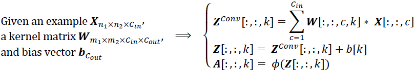
Equation 14-1 summarizes the preceding explanations in one big mathematical equation: it shows how to compute the output of a given neuron in a convolutional layer. It is a bit ugly丑陋 due to all the different indices, but all it does is calculate the weighted sum of all the inputs, plus the bias term.
Equation 14-1. Computing the output of a neuron in a convolutional layer
 <==~ or v: from 0 to fw -1 ; u: from 0 to fh -1
#############

 https://blog.csdn.net/Linli522362242/article/details/108414534
If there is only one layer of feature map before( =1), then the sum of the results obtained by multiplying(element-wise multiplication) a receptive field (a matrix containing the values of cells in a specific range (v: from 0 to fw -1 ; u: from 0 to fh -1)) in the previous feature map(k′) by the weight matrix(
 x
x ) plus the bias of the current feature map(k) is the current output
 of at cell( i,j ) in the current feature map(k)
the weight matrix plus the bias : all neurons within a given feature map share the same parameters (i.e., the same weights and bias term)
#############
In this equation:
-
is the output of the neuron located in row i, column j in feature map k of the convolutional layer (layer L).
- As explained earlier,
 and
and  are the vertical and horizontal strides, and are the height and width of the receptive field, and is the number of feature maps in the previous layer (layer L – 1).
-
 is the output of the neuron located in layer L – 1, row i′, column j′, feature map k′ (or channel k′ if the previous layer is the input layer).
-
 is the bias term for feature map k (in layer L). You can think of it as a knob that tweaks the overall brightness of the feature map k.
-
 is the connection weight between any neuron in feature map k of the layer L and its input located at row u, column v its input located at row u, column v (relative to the neuron’s receptive field in all feature maps of previous layer L – 1), and feature map k′.
TensorFlow Implementation
In TensorFlow, each input image is typically represented as a 3D tensor of shape [height, width, channels]. A mini-batch is represented as a 4D tensor of shape [minibatch size, height, width, channels]. The weights of a convolutional layer are represented as a 4D tensor of shape  . The bias terms of a convolutional layer are simply represented as a 1D tensor of shape
  .
.
Let’s look at a simple example. The following code loads two sample images, using Scikit-Learn’s load_sample_image() (which loads two color images, one of a Chinese temple, and the other of a flower), then it creates two filters and applies them to both images, and finally it displays one of the resulting feature maps. Note that you must pip install the Pillow package to use load_sample_image().
- images is the input mini-batch (a 4D tensor, as explained earlier). #( batch_size, height, width, channels )
- filters is the set of filters to apply (also a 4D tensor, as explained earlier).
and are the height and width of the receptive field
fh=7(height), fw=7(width), fn′=3 (number of feature maps or channels in the previous layer (layer L – 1) ), filters=2 (number of feature maps)
import numpy as np
from sklearn.datasets import load_sample_image

# scale these features simply by dividing by 255, to get floats ranging from 0 to 1.
china = load_sample_image("china.jpg") / 255   # china.shape: (427, 640, 3)
flower = load_sample_image("flower.jpg") / 255 # flower.shape: (427, 640, 3)
images = np.array([china, flower])  # images.shape: (2, 427, 640, 3)
batch_size, height, width, channels = images.shape

# Create 2 filters
# fh=7(height), fw=7(width), fn′=3 (number of feature maps or filters in previous layer),2 filters
filters = np.zeros( shape=(7,7, channels, 2), dtype=np.float32 )
 # 7,[...,3,...],3, 0
filters[:, 3, :, 0] = 1 #creates a vertical line uses filters[0] # vertical filter
 # [...,3,...],7,3,1
filters[3, :, :, 1] = 1 #creates a horizontal line uses filters[1] # horizontal filter
filters.shape : (7, 7, 3, 2):
filters

... ...(7,7, 3,2)

The tf.nn.conv2d() line deserves a bit more explanation:
padding must be either "SAME" or "VALID":
- —If set to "SAME", the convolutional layer uses zero padding if necessary. The output size is set to the number of input neurons divided by the stride, rounded up. For example, if the input size is 13 and the stride is 5 (see Figure 14-7), then the output size is 3 (i.e., 13 / 5 = 2.6, rounded up to 3 or ceil(13/5)= 3). Then zeros are added as evenly as possible around the inputs, as needed. When strides=1, the layer’s outputs will have the same spatial dimensions (width and height) as its inputs, hence the name same.

- —If set to "VALID", the convolutional layer does not use zero padding and may ignore some rows and columns at the bottom and right of the input image, depending on the stride, as shown in Figure 14-7 (for simplicity, only the horizontal dimension is shown here, but of course the same logic applies to the vertical dimension垂直尺寸也适用相同的逻辑). This means that every neuron’s receptive field lies strictly within valid positions inside the input (it does not go out of bounds), hence the name valid.

import matplotlib.pyplot as plt

# strides=1 or [1,sh,sw,1]
# [1,sh(vertical stride), sw(horizontal stride),1]
# The first and last elements must currently be equal to 1. They may one day be used to
# specify a batch stride (to skip some instances) and a channel stride (to skip some
# of the previous layer’s feature maps or channels)
outputs = tf.nn.conv2d(images, filters, strides=1, padding="SAME")
#return a feature maps
# outputs.shape: TensorShape([2, 427, 640, 2]) # #( batch_size, height, width, channels )

plt.imshow(outputs[0,:,:,1], cmap="gray") # # plot 1st image's 2nd feature map #horizontal filter
plt.axis("off")
plt.show()

outputs.shape

 =
=
input_shape from images.shape: (2 batches, 427, 640, 3) ==> each batch * ( m_1(or f_h)=7, m_2(or f_w)=7, C_in=3, C_out =2 ) or and strides=1, padding="SAME") ==> TensorShape([2 batches, 427, 640, 2]): [batch size, height, width, num_channels or num_filters or C_out ]
<== for every cell in each C_out : 
is the output of the neuron located in layer L – 1, row i′, column j′, feature map k′ (or channel k′ if the previous layer is the input layer).
v: from 0 to fw -1 ; u: from 0 to fh -1 (relative to the neuron’s receptive field, s_h=1: stride on horizontal direction, s_w=1: stride on vertical direction)
is the connection weight between any neuron in feature map k of the layer L and its input located at row u, column v (relative to the neuron’s receptive field in all feature maps of previous layer L – 1), and feature map k′ (here is from 0 to 3-1).
 the current feature map index: k
plt.imshow(outputs[0,:,:,0], cmap="gray") # # plot 1st image's 1st feature map #vertical filter
plt.axis("off")
plt.show()

plt.imshow(china, cmap="gray") # # plot 1st image's 2nd feature map
plt.axis("off")
plt.show()

Let’s go through this code:
- The pixel intensity for each color channel is represented as a byte from 0 to 255, so we scale these features simply by dividing by 255, to get floats ranging from 0 to 1. ### china = load_sample_image("china.jpg") / 255
- Then we create two 7 × 7 filters ### filters = np.zeros( shape=(7,7, channels, 2), dtype=np.float32 )
( one with a vertical white line in the middle, ### filters[:, 3, :, 0] = 1
and the other with a horizontal white line in the middle ### filters[3, :, :, 1] = 1 ).
- We apply them to both images using the tf.nn.conv2d() function, which is part of TensorFlow’s low-level Deep Learning API. In this example, we use zero padding (padding="SAME") and a stride of 1.
### outputs = tf.nn.conv2d(images, filters, strides=1, padding="SAME")
- Finally, we plot one of the resulting feature maps (similar to the top-right image in Figure 14-5).
### plt.imshow(outputs[0,:,:,1], cmap="gray") # plot 1st image's 2nd feature map # horizontal filter
def plot_image(image):
    plt.imshow(image, cmap="gray", interpolation="nearest")
    plt.axis("off")
for image_index in(0,1): #0:Chinese temple, 1: flower
    for feature_map_index in (0,1): # 0: vertical filter # 1: horizontal filter
        plt.subplot(2,2, image_index*2 +feature_map_index +1)
        plot_image( outputs[image_index,:,:, feature_map_index])

plt.show()

def crop(images):
    return images[150:220, 130:250]

print("Chinese_Temple_Original_Cropped")
plot_image( crop(images[0, :,:, 0]) )
plt.show()

for feature_map_index, filename in enumerate( ["china_vertical", "china_horizontal"] ):
    print(filename)
    plot_image( crop( outputs[0,:,:, feature_map_index] ) ) # #( batch_size, height, width, channels )
    plt.show()
 ==>
==>
plot_image(filters[:, :, 0, 0]) # (7,7, channels, 2)
plt.show()
plot_image(filters[:, :, 0, 1])
plt.show()

In this example we manually defined the filters, but in a real CNN you would normally define filters as trainable variables so the neural net can learn which filters work best, as explained earlier. Instead of manually creating the variables, use the keras.layers.Conv2D layer:
from tensorflow import keras

conv = keras.layers.Conv2D( filters=32, kernel_size=3, strides=1, padding='SAME',
                            activation='relu' ) # return ( batch_size, height, width, channels )
This code creates a Conv2D layer with 32 filters, each 3 × 3, using a stride of 1 (both horizontally and vertically) and "same" padding, and applying the ReLU activation function to its outputs. As you can see, convolutional layers have quite a few hyperparameters: you must choose the number of filters, their height and width, the strides, and the padding type. As always, you can use cross-validation to find the right hyperparameter values, but this is very time-consuming. We will discuss common CNN architectures later, to give you some idea of which hyperparameter values work best in practice.
Memory Requirements
Another problem with CNNs is that the convolutional layers require a huge amount of RAM. This is especially true during training, because the reverse pass of backpropagation requires all the intermediate values computed during the forward pass.
 A fully connected layer ( top: neurons on current layer, botton: neurons on previous layer
For example, consider a convolutional layer with 5 × 5 ( == x ) filters, outputting 200 feature maps of size 150 × 100, with stride 1 and "same" padding. If the input is a 150 × 100 RGB image (three channels), then the number of parameters is (5 × 5 × 3 + 1) × 200 = 15,200 (the + 1 corresponds to the bias terms, and 3 possible sets of weights), which is fairly small compared to a fully connected layer(A fully connected layer with 150 × 100 neurons, each connected to all 150 × 100 × 3 inputs, would have 150^2× 100^2 × 3 = 675 million(OR 675,000,000) parameters!). However, each of the 200 feature maps(output) contains 150 × 100 neurons, and each of these neurons needs to compute a weighted sum of its 5 × 5 × 3 = 75 inputs: that’s a total of 225 million float multiplications(225, 000, 000=75 inputs * 150*100 neurons*200 feature maps). Not as bad as a fully connected layer, but still quite computationally intensive(for convolutional layer). Moreover, if the feature maps are represented using 32-bit floats, then the convolutional layer’s output will occupy 200 × 150 × 100 × 32 = 96 million bits (12 MB) of RAM(In the international system of units (SI), 1 MB = 1,000 KB = 1,000 × 1,000 bytes = 1,000 × 1,000 × 8 bits.). And that’s just for one instance—if a training batch contains 100 instances, then this layer will use up 1.2 GB of RAM!
During inference (i.e., when making a prediction for a new instance) the RAM occupied by one layer can be released as soon as the next layer has been computed, so you only need as much RAM as required by two consecutive layers. But during training everything computed during the forward pass needs to be preserved for the reverse pass, so the amount of RAM needed is (at least) the total amount of RAM required by all layers.
If training crashes because of an out-of-memory error, you can try reducing the mini-batch size. Alternatively, you can try reducing dimensionality using a stride, or removing a few layers. Or you can try using 16-bit floats instead of 32-bit floats. Or you could distribute the CNN across multiple devices.
Now let’s look at the second common building block of CNNs: the pooling layer.
Pooling Layers
Once you understand how convolutional layers work, the pooling layers are quite easy to grasp. Their goal is to subsample (i.e., shrink) the input image in order to reduce the computational load, the memory usage, and the number of parameters (thereby limiting the risk of overfitting).
 Figure 14-8. Max pooling layer (2 × 2 pooling kernel, stride 2, no padding)
Just like in convolutional layers, each neuron in a pooling layer is connected to the outputs of a limited number of neurons in the previous layer, located within a small rectangular receptive field. You must define its size, the stride, and the padding type, just like before. However, a pooling neuron has no weights; all it does is aggregate the inputs using an aggregation function such as the max or mean. Figure 14-8 shows a max pooling layer, which is the most common type of pooling layer. In this example, we use a 2 × 2 pooling kernel, with a stride of 2 and no padding. Only the max input value in each receptive field makes it to the next layer, while the other inputs are dropped. For example, in the lower-left receptive field in Figure 14-8, the input values are 1, 5, 3, 2, so only the max value, 5, is propagated to the next layer. Because of the stride of 2, the output image has half the height and half the width of the input image (rounded down since we use no padding).
A pooling layer typically works on every input channel independently, so the output depth is the same as the input depth.
 Figure 14-9. Invariance to small translations
Other than reducing computations, memory usage, and the number of parameters, a max pooling layer also introduces some level of invariance不变性 to small translations, as shown in Figure 14-9. Here we assume that the bright pixels have a lower value than dark pixels, and we consider three images (A, B, C) going through a max pooling layer with a 2 × 2 kernel and stride 2. Images B and C are the same as image A, but shifted by one and two pixels to the right. As you can see, the outputs of the max pooling layer for images A and B are identical. This is what translation invariance means. For image C, the output is different: it is shifted one pixel to the right (but there is still 75% invariance). By inserting a max pooling layer every few layers in a CNN, it is possible to get some level of translation invariance at a larger scale. Moreover, max pooling offers a small amount of rotational invariance and a slight scale invariance. Such invariance (even if it is limited) can be useful in cases where the prediction should not depend on these details, such as in classification tasks.
However, max pooling has some downsides too . Firstly, it is obviously very destructive破坏性的: even with a tiny 2 × 2 kernel and a stride of 2, the output will be two times smaller in both directions (so its area will be four times smaller), simply dropping 75% of the input values (1-4x4/(8x8)=1-0.25=0.75). And in some applications, invariance is not desirable. Take semantic segmentation (the task of classifying each pixel in an image according to the object that pixel belongs to, which we’ll explore later in this chapter): obviously, if the input image is translated by one pixel to the right, the output should also be translated by one pixel to the right. The goal in this case is equivariance, not invariance: a small change to the inputs should lead to a corresponding small change in the output.
TensorFlow Implementation
Implementing a max pooling layer in TensorFlow is quite easy. The following code creates a max pooling layer using a 2 × 2 kernel. The strides default to the kernel size, so this layer will use a stride of 2 (both horizontally and vertically). By default, it uses "valid" padding (i.e., no padding at all):
To create an average pooling layer, just use AvgPool2D instead of MaxPool2D. As you might expect, it works exactly like a max pooling layer, except it computes the mean rather than the max. Average pooling layers used to be very popular, but people mostly use max pooling layers now, as they generally perform better. This may seem surprising, since computing the mean generally loses less information than computing the max. But on the other hand, max pooling preserves only the strongest features, getting rid of all the meaningless ones, so the next layers get a cleaner signal to work with. Moreover, max pooling offers stronger translation invariance than average pooling, and it requires slightly less compute.
 Figure 14-10. Depthwise max pooling can help the CNN learn any invariance
Note that max pooling and average pooling can be performed along the depth dimension rather than the spatial空间 dimensions, although this is not as common. This can allow the CNN to learn to be invariant to various features. For example, it could learn multiple filters, each detecting a different rotation of the same pattern (such as handwritten digits### 3 OR 6; see Figure 14-10), and the depthwise深度 max pooling layer would ensure that the output is the same regardless of the rotation. The CNN could similarly learn to be invariant to anything else: thickness, brightness, skew, color, and so on.
MaxPooling2D layer
#######################################################################
tf.keras.layers.MaxPooling2D(
    pool_size=(2, 2), strides=None, padding="valid", data_format=None, **kwargs
)
x = tf.constant([[1., 2., 3.],
                 [4., 5., 6.],
                 [7., 8., 9.]
                ]) # x.shape : TensorShape([3, 3])
#                 ( batch_size, height, width, channels )
x = tf.reshape(x, [1,3,3,1])
# x
# <tf.Tensor: shape=(1, 3, 3, 1), dtype=float32, numpy=
# array([
#         [ # (1, 3)
#           [[1.], # (3,1)
#            [2.],
#            [3.]
#           ],

#           [[4.], # (3,1)
#            [5.],
#            [6.]
#           ],

#           [[7.], # (3,1)
#            [8.],
#            [9.]
#           ]
#        ] # (1, 3)
#      ], dtype=float32)>
#tf.keras.layers.MaxPool2D <== Main aliases ==> tf.keras.layers.MaxPooling2D
max_pool_2d = tf.keras.layers.MaxPooling2D( pool_size=(2,2), # OR pool_size=2
                                            strides = (1,1), # OR strides = 1
                                            padding='valid'
                                          )
                # output_shape = ceil(input_shape - pool_size + 1) / strides # using "valid"
max_pool_2d(x)  # output_shape = ceil( (3,3) - (2,2) + 1) / (1,1) ) ==> (2,2)
 output_shape = ceil( (3,3) - (2,2) + 1) / (1,1) ) OR n(3,3) +2* p(0,0) - f(2,2) / s(1,1) +(1,1) ==> (2,2)
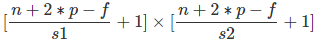
特征图的行列数计算公式:
对于n*n的矩阵, 使用 f*f 的核进行卷积, 填充宽度为p, 若纵向步幅为s1, 横向步幅为s2则特征图的行列数为:
x = tf.constant([[1., 2., 3., 4.],
                 [5., 6., 7., 8.],
                 [9., 10., 11., 12.]
                ]) # strides=(2, 2) and using "valid" will ignore last row in x
# x.shape : TensorShape([3, 4])
#                 ( batch_size, height, width, channels )
x = tf.reshape(x, [1, 3, 4, 1])
max_pool_2d = tf.keras.layers.MaxPooling2D(pool_size=(2, 2),
                                           strides=(2, 2),
                                           padding='valid'
                                          )
            # output_shape = (input_shape - pool_size + 1) / strides # using "valid"
max_pool_2d(x) # output_shape = ceil( (3,4) - (2,2) + 1 ) / (2,2) ) ==> (1,2)
 output_shape = ceil( (3,4) - (2,2) + 1 ) / (2,2) ) OR OR n (3,4) +2* p(0,0) - f(2,2) / s (2,2) +(1,1) ==> (1,2)
#######################################################################
import matplotlib as mpl

# def crop(images):
#     return images[150:220, 130:250]

max_pool = keras.layers.MaxPool2D( pool_size=2 ) # OR pool_size=(2,2)

#images = np.array([china, flower])  # images.shape: (2, 427, 640, 3)
cropped_images = np.array([ crop(image) for image in images ], dtype=np.float32) #since tf using 64
output = max_pool( cropped_images )

fig = plt.figure( figsize=(12,8) )

# matplotlib.gridspec.GridSpec
# A grid layout to place subplots within a figure.
# width_ratios: array-like of length ncols, optional
              # Defines the relative widths of the columns.
              # Each column gets a relative width of width_ratios[i] / sum(width_ratios).
              # If not given, all columns will have the same width.
gs = mpl.gridspec.GridSpec( nrows=1, ncols=2, width_ratios=[2,1] )

ax1 = fig.add_subplot( gs[0,0] )
ax1.set_title("Input", fontsize=14)
ax1.imshow( cropped_images[0] ) # plot the 1st image
ax1.axis("off")

ax2 = fig.add_subplot( gs[0,1] )
ax2.set_title("Output", fontsize=14)
ax2.imshow( output[0] )
ax2.axis("off")

plt.show()

Depth-wise pooling
##############################################################
tf.nn.max_pool(
    input, ksize, strides, padding, data_format=None, name=None
)
input: #( batch_size, height, width, channels )
Tensor of rank N+2, of shape `[batch_size] + input_spatial_shape + [num_channels]` if `data_format` does not start with "NC" (default),
or `[batch_size, num_channels] + input_spatial_shape` if data_format starts with "NC".
Pooling happens over the spatial dimensions only.
ksize: An int or list of ints that has length 1, N or N+2. The size of the window for each dimension of the input tensor.
strides: An int or list of ints that has length 1, N or N+2. The stride of the sliding window for each dimension of the input tensor.
padding: A string, either 'VALID' or 'SAME'. The padding algorithm. See the "returns" section of tf.nn.convolution for details.
data_format: A string. Specifies the channel dimension. For N=1 it can be either "NWC" (default) or "NCW", for N=2 it can be either "NHWC" (default) or "NCHW" and for N=3 either "NDHWC" (default) or "NCDHW".
NHWC: N~batch_size, H~Height, W~Width, C~Channels
name: Optional name for the operation.
Returns: A Tensor of format specified by data_format. The max pooled output tensor.
a = tf.constant([
    [[1.0, 2.0, 3.0, 4.0],
     [5.0, 6.0, 7.0, 8.0],
     [8.0, 7.0, 6.0, 5.0],
     [4.0, 3.0, 2.0, 1.0]],
    [[4.0, 3.0, 2.0, 1.0],
     [8.0, 7.0, 6.0, 5.0],
     [1.0, 2.0, 3.0, 4.0],
     [5.0, 6.0, 7.0, 8.0]]
])
a

a_new = tf.reshape(a, [1,4,4,2]) # (batch_size, height, width, channels)
a_new # 1 x (4 x (4,2) )
red : channel 1
blue : channel 2
 <==>
<==>
uses k_size=[1,2,2,1], strides=[1,1,1,1] iterates a_new 2 channels ,respects : kernel size=(2,2) and stride size=(1,1) you want along the spatial dimensions (height and width) in each channel (or each feature map since a divisor of the input depth=1)

 ,
, 
 ,
, 

==> 
First, perform max_pool on the first two columns(since f_h=2) of the first channel and the first two rows(since f_w=2)  to get the value 8.
Then perform max_pool on the first two columns(since f_h=2) of the second channel and the first two rows(since f_w=2)  to get the value 7,
after traversing the first two rows, then perform max_pool on the first two columns on the middle two rows of the first channel  to get the value 6, so on
# along the spatial dimensions (height and width, k_size=[1,2,2,1] and strides=[1,1,1,1] : kernel size=(2,2) stride size=(1,1) ) in each channel (or each feature map since a divisor of the input depth=1)
pooling=tf.nn.max_pool(a_new,             # [batch_size, height, width, channels]
                       ksize=[1,2,2,1],   # [1, f_height, f_width, 1]
                       strides=[1,1,1,1], # [1, stride,stride, 1]
                       padding='VALID')
pooling # output_shape = (input_shape - pool_size + 1) / strides # using "valid"
        # output_shape = ( (4,4) - (2,2) +1 ) / 1 = (3, 3)
        # final output shape = (batch_size=1, 3,3, channels=2)

The ksize argument contains the kernel shape along all four dimensions of the input tensor: [batch size, height, width, channels]. TensorFlow currently does not support pooling over multiple instances, so the first element of ksize must be equal to 1. Moreover, it does not support pooling over both the spatial dimensions (height and width) and the depth dimension, so either ksize[1] and ksize[2] must both be equal to 1, or ksize[3] must be equal to 1.
##############################################################
Keras does not include a depthwise max pooling layer, but TensorFlow’s low-level Deep Learning API does: just use the tf.nn.max_pool() function, and specify the kernel size and strides as 4-tuples (i.e., tuples of size 4). The first three values of each should be 1: this indicates that the kernel size and stride along the batch, height, and width dimensions should be 1. The last value should be whatever kernel size and stride you want along the depth dimension—for example, 3 (this must be a divisor of the input depth; it will not work if the previous layer outputs 20 feature maps, since 20 is not a multiple of 3):
output = tf.nn.max_pool(images,
                        ksize=(1, 1, 1, 3),
                        strides=(1, 1, 1, 3),
                        padding="valid")
# along the depth dimension ( k_size=(1, 1, 1, 3) and strides=(1, 1, 1, 3) : kernel size=(1,1) stride size=(1,1) ) with a divisor of the input depth=3
# def crop(images):
#     return images[150:220, 130:250] ### ==> 70,120

# images = np.array([china, flower])  # images.shape: (2, 427, 640, 3)
# cropped_images = np.array([ crop(image) for image in images ], dtype=np.float32) #since tf using 64

class DepthMaxPool(keras.layers.Layer):
    def __init__(self, pool_size, strides=None, padding="VALID", **kwargs):
        super().__init__(**kwargs)
        if strides is None:
            strides = pool_size
        self.pool_size = pool_size
        self.strides = strides
        self.padding = padding

    def call(self, inputs):
        # if input.shape is not None: # input.shape : (70, 120)
        #    n = len(input.shape) - 2
        # elif data_format is not None:
        #    n = len(data_format) - 2
        return tf.nn.max_pool(inputs,
                              ksize=(1,1,1, self.pool_size),
                              strides=(1,1,1, self.strides),
                              padding=self.padding)

depth_pool = DepthMaxPool(3) #channels=3
with tf.device("/cpu:0"): # there is no GPU-kernel yet
    depth_output = depth_pool(cropped_images)
depth_output.shape
 : for a rgb image input depth=3, here the divisor of the input depth=3, 3/3=1
If you want to include this as a layer in your Keras models, wrap it in a Lambda layer (or create a custom Keras layer):
depth_pool = keras.layers.Lambda( lambda X: tf.nn.max_pool(
    X, ksize=(1,1,1,3), strides=(1,1,1,3), padding="VALID"
    ))
with tf.device("/cpu:0"):
    depth_output = depth_pool(cropped_images)
depth_output.shape

tf.nn,tf.layers, tf.contrib模块有很多功能是重复的
下面是对三个模块的简述:
- tf.nn :提供神经网络相关操作的支持,包括卷积操作(conv)、池化操作(pooling)、归一化、loss、分类操作、embedding、RNN、Evaluation。
- tf.layers:主要提供的高层的神经网络,主要和卷积相关的,tf.nn会更底层一些。
- tf.contrib:tf.contrib.layers提供够将计算图中的 网络层、正则化、摘要操作、是构建计算图的高级操作,但是tf.contrib包含不稳定和实验代码,有可能以后API会改变。
def plot_color_image(image):
    plt.imshow(image, interpolation="nearest")
    plt.axis("off")

def plot_image(image):
    plt.imshow(image, cmap="gray", interpolation="nearest")
    plt.axis("off")

plt.figure(figsize=(12,8))

plt.subplot(1,2,1)
plt.title("Input", fontsize=14)
plot_color_image( cropped_images[0] ) # plot the 1st image

plt.subplot(1,2,2)
plt.title("Output", fontsize=14)
plot_image( depth_output[0, ..., 0]) # plot the output for the 1st image

#plt.axis("off")
plt.show(

One last type of pooling layer that you will often see in modern architectures is the global average pooling layer. It works very differently: all it does is compute the mean of each entire feature map (it’s like an average pooling layer using a pooling kernel with the same spatial dimensions as the inputs). This means that it just outputs a single number per feature map and per instance. Although this is of course extremely destructive (most of the information in the feature map is lost), it can be useful as the output layer, as we will see later in this chapter. To create such a layer, simply use the keras.layers.GlobalAvgPool2D class:
global_avg_pool = keras.layers.GlobalAvgPool2D()
global_avg_pool(cropped_images)

cropped_images.shape

It’s equivalent to this simple Lambda layer, which computes the mean over the spatial dimensions (height and width):
output_global_avg2 = keras.layers.Lambda( lambda X: tf.reduce_mean(X, axis=[1,2]) )
output_global_avg2(cropped_images)

Now you know all the building blocks to create convolutional neural networks. Let’s see how to assemble them.
CNN Architectures
Typical CNN architectures stack a few convolutional layers (each one generally followed by a ReLU layer), then a pooling layer, then another few convolutional layers (+ReLU), then another pooling layer, and so on. The image gets smaller and smaller as it progresses through the network, but it also typically gets deeper and deeper (i.e., with more feature maps), thanks to the convolutional layers (see Figure 14-11). At the top of the stack, a regular feedforward neural network is added, composed of a few fully connected layers (+ReLUs), and the final layer outputs the prediction (e.g., a softmax layer that outputs estimated class probabilities).
 Figure 14-11. Typical CNN architecture
A common mistake is to use convolution kernels that are too large. For example, instead of using a convolutional layer with a 5 × 5 kernel, stack two layers with 3 × 3 kernels: it will use fewer parameters and require fewer computations, and it will usually perform better. One exception is for the first convolutional layer: it can typically have a large kernel (e.g., 5 × 5), usually with a stride of 2 or more: this will reduce the spatial dimension of the image without losing too much information, and since the input image only has three channels in general, it will not be too costly.
Here is how you can implement a simple CNN to tackle the Fashion MNIST dataset (introduced in Chapter 10):
from tensorflow import keras
import numpy as np

(X_train_full, y_train_full), (X_test, y_test) = keras.datasets.fashion_mnist.load_data()
X_train, X_valid = X_train_full[:-5000], X_train_full[-5000:]
y_train, y_valid = y_train_full[:-5000], y_train_full[-5000:]

# X_train.shape # (55000, 28, 28)
# X_valid.shape # (5000, 28, 28)
# X_test.shape # (10000, 28, 28)

X_mean = X_train.mean(axis=0, keepdims=True) # get each feature's average
# X_mean.shape # (1, 28, 28)
X_std = X_train.std(axis=0, keepdims=True) + 1e-7
X_train = (X_train-X_mean) / X_std # standardization
X_valid = (X_valid-X_mean) / X_std
X_test = (X_test-X_mean) / X_std

X_train = X_train[..., np.newaxis] # ==>( batch_size, height, width, channels )
# X_train.shape # (55000, 28, 28, 1)
X_valid = X_valid[..., np.newaxis]
X_test = X_test[..., np.newaxis]
print(X_train.shape)

from functools import partial

# tf.keras.layers.Conv2D(
#     filters, kernel_size, strides=(1, 1), padding='valid', data_format=None,
#     dilation_rate=(1, 1), groups=1, activation=None, use_bias=True,
#     kernel_initializer='glorot_uniform', bias_initializer='zeros',
#     kernel_regularizer=None, bias_regularizer=None, activity_regularizer=None,
#     kernel_constraint=None, bias_constraint=None, **kwargs
# )
# kernel_size : An integer or tuple/list of 2 integers, specifying the height and width
#               of the 2D convolution window. Can be a single integer to specify the same
#               value for all spatial dimensions.
DefaultConv2D = partial( keras.layers.Conv2D,
                         kernel_size = 3, #(3,3) #  convolution kernels OR filters
                         activation="relu",
                         padding="SAME"
                       )

model = keras.models.Sequential([
    DefaultConv2D(filters=64, # 64 filters OR 64 feature maps OR 64 possible sets of weights
                  kernel_size=7, # filter
                  input_shape=[28,28,1]),
    keras.layers.MaxPooling2D(pool_size=2),#Max since the classification

    DefaultConv2D(filters=128),
    DefaultConv2D(filters=128),
    keras.layers.MaxPooling2D(pool_size=2),

    DefaultConv2D(filters=256),
    DefaultConv2D(filters=256),
    keras.layers.MaxPooling2D(pool_size=2),

    keras.layers.Flatten(), # to 1D since using Dense
    keras.layers.Dense(units=128, activation='relu'),
                        # dropout rate closer to 40–50% in convolutional neural networks
    keras.layers.Dropout(0.5), # being less sensitive to slight changes in the inputs
    keras.layers.Dense(units=64, activation='relu'),
                        # resulting neural network can be seen as an averaging ensemble
    keras.layers.Dropout(0.5), # of all these smaller neural networks
    keras.layers.Dense(units=10, activation='softmax'), # 10 categories
])
Let’s go through this model:
- The first layer uses 64 fairly large filters (7 × 7) but no stride because the input images are not very large. It also sets input_shape=[28, 28, 1], because the images are 28 × 28 pixels, with a single color channel (i.e., grayscale).
- Next we have a max pooling layer which uses a pool size of 2, so it divides each spatial dimension by a factor of 2. (28/2==14)
- Then we repeat the same structure twice: two convolutional layers followed by a max pooling layer. For larger images, we could repeat this structure several more times (the number of repetitions is a hyperparameter you can tune).
- Note that the number of filters grows as we climb up the CNN toward the output layer (it is initially 64, then 128, then 256): it makes sense for it to grow, since the number of low-level features is often fairly low (e.g., small circles, horizontal lines), but there are many different ways to combine them into higher-level features.
It is a common practice to double the number of filters after each pooling layer: since a pooling layer divides each spatial dimension by a factor of 2, we can afford to double the number of feature maps in the next layer without fear of exploding the number of parameters, memory usage, or computational load.
- Next is the fully connected network, composed of two hidden dense layers and a dense output layer. Note that we must flatten its inputs, since a dense network expects a 1D array of features for each instance. We also add two dropout layers, with a dropout rate of 50% each, to reduce overfitting.
model.compile( loss="sparse_categorical_crossentropy",
               optimizer='nadam',
               metrics=["accuracy"])
history = model.fit(X_train, y_train, epochs=10, validation_data=(X_valid, y_valid))
score = model.evaluate(X_test, y_test)
X_new = X_test[:10] # pretend we have new images
y_pred = model.predict(X_new)
print(score)
https://colab.research.google.com/drive/1HEwjeJWOyPU3GltaqnuublqXmvjrx76t#scrollTo=mnPK3Dm_mMA7

OR https://colab.research.google.com/drive/1HEwjeJWOyPU3GltaqnuublqXmvjrx76t#scrollTo=lLgKIS2UmF0B

import math

math.ceil(55000/history.params["batch_size"])
 =55000/32(default) and 333=10000/32
This CNN reaches over 90% accuracy on the test set. It’s not state of the art, but it is pretty good, and clearly much better than what we achieved with dense networks in Chapter 10 https://blog.csdn.net/Linli522362242/article/details/106562190 .
.
Over the years, variants of this fundamental architecture have been developed, leading to amazing advances in the field. A good measure of this progress is the error rate in competitions such as the ILSVRC ImageNet challenge. In this competition the topfive error rate for image classification fell from over 26% to less than 2.3% in just six years. The top-five error rate is the number of test images for which the system’s top five predictions did not include the correct answer. The images are large (256 pixels high) and there are 1,000 classes, some of which are really subtle (try distinguishing 120 dog breeds). Looking at the evolution of the winning entries is a good way to understand how CNNs work.
We will first look at the classical LeNet-5 architecture (1998), then three of the winners of the ILSVRC challenge: AlexNet (2012), GoogLeNet (2014), and ResNet (2015).
LeNet-5
https://blog.csdn.net/Linli522362242/article/details/108396485