以下代码来自Deep Learning for Computer Vision with Python第九章。
一、梯度下降法(Gradient Decent)
# import the necessary packages
from sklearn.model_selection import train_test_split
from sklearn.metrics import classification_report
from sklearn.datasets import make_blobs
import matplotlib.pyplot as plt
import numpy as np
import argparse

def sigmoid_activation(x):
	# compute the sigmoid activation value for a given input
	return 1.0 / (1 + np.exp(-x))

def predict(X, W):
	# take the dot product between our features and weight matrix
	preds = sigmoid_activation(X.dot(W))

	# apply a step function to threshold the outputs to binary
	# class labels
	preds[preds <= 0.5] = 0
	preds[preds > 0] = 1

	# return the predictions
	return preds

# construct the argument parse and parse the arguments
ap = argparse.ArgumentParser()
ap.add_argument("-e", "--epochs", type=float, default=100,
	help="# of epochs")
ap.add_argument("-a", "--alpha", type=float, default=0.01,
	help="learning rate")
args = vars(ap.parse_args())

# generate a 2-class classification problem with 1,000 data points,
# where each data point is a 2D feature vector
(X, y) = make_blobs(n_samples=1000, n_features=2, centers=2,
	cluster_std=1.5, random_state=1)
y = y.reshape((y.shape[0], 1))

# insert a column of 1's as the last entry in the feature
# matrix -- this little trick allows us to treat the bias
# as a trainable parameter within the weight matrix
X = np.c_[X, np.ones((X.shape[0]))]

# partition the data into training and testing splits using 50% of
# the data for training and the remaining 50% for testing
(trainX, testX, trainY, testY) = train_test_split(X, y,
	test_size=0.5, random_state=42)

# initialize our weight matrix and list of losses
print("[INFO] training...")
W = np.random.randn(X.shape[1], 1)
losses = []

# loop over the desired number of epochs
for epoch in np.arange(0, args["epochs"]):
	# take the dot product between our features 'X' and the weight
	# matrix 'W', then pass this value through our sigmoid activation
	# function, thereby giving us our predictions on the dataset
	preds = sigmoid_activation(trainX.dot(W))

	# now that we have our predictions, we need to determine the
	# 'error', which is the difference between our predictions and
	# the true values
	error = preds - trainY
	loss = np.sum(error ** 2)
	losses.append(loss)

	# the gradient descent update is the dot product between our
	# features and the error of the predictions
	gradient = trainX.T.dot(error)

	# in the update stage, all we need to do is "nudge" the weight
	# matrix in the negative direction of the gradient (hence the
	# term "gradient descent" by taking a small step towards a set
	# of "more optimal" parameters
	W += -args["alpha"] * gradient

	# check to see if an update should be displayed
	if epoch == 0 or (epoch + 1) % 5 == 0:
		print("[INFO] epoch={}, loss={:.7f}".format(int(epoch + 1),
			loss))

# evaluate our model
print("[INFO] evaluating...")
preds = predict(testX, W)
print(classification_report(testY, preds))

# plot the (testing) classification data
plt.style.use("ggplot")
plt.figure()
plt.title("Data")
plt.scatter(testX[:, 0], testX[:, 1], marker="o", c=testY, s=30)

# construct a figure that plots the loss over time
plt.style.use("ggplot")
plt.figure()
plt.plot(np.arange(0, args["epochs"]), losses)
plt.title("Training Loss")
plt.xlabel("Epoch #")
plt.ylabel("Loss")
plt.show()
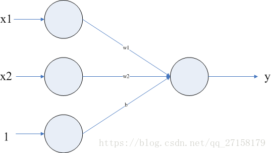
本例子的神经网络是只有两层,输入3,输出1,(3-1)。且输入3个神经元中,最后一个是输入为1。是为了将偏移(bias)b值放到权重矩阵W中。
Python语言,使用了sklearn、matplotlib、numpy、imutils这几个库。
这个例程中,学习的内容如下:
1、细胞元激活函数
本例子采用sigmoid函数。
sigmoid函数曲线如下:
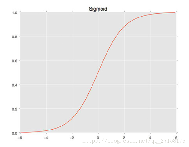
理论上,神经网络中每个神经元只有两种状态:有反应、无反应,即1和0。但这里允许神经元具有0-1V之间的任意电压。且输入输出符合Sigmoid曲线。
2、predict预测函数
预测函数中,把输入的变量X(3行1列矩阵)经过转置变成1行3列,乘以权值W(3行1列),得到输出。
3、网络初始化
使用make_blobs函数生成了1000个样品,每个样品两个参数。即输入矩阵是1000行2列。输出只有一个参数,是1行1000列。
X = np.c_[X, np.ones((X.shape[0]))]这语句可以在输入矩阵最低加上一行1,同时把权值W(weights)矩阵初始化为3行1列,最后1列是偏置b(bias)。
线性分类基本公式是:
可以把b放进权重W矩阵的最后一行,这样的好处是,可以在训练W矩阵时,也训练了b参数。
train_test_split函数可以将样品(X,y)按比例分配成一部分用于训练,一部分用于测试。
4、网络训练
这例子,更新权重矩阵W的频率是把全部训练样品处理一次,才更新一次的权重。因此学习速度十分缓慢。
error是全部训练样品的预测结果,和实际结果y想减。
损失函数是error中每个元素的平方和:loss = np.sum(error ** 2)
更新权值的公式是
error = preds - trainY
gradient = trainX.T.dot(error)
W += -args["alpha"] * gradient
5、网络测试
测试使用了classification_report.第一个参数是实际值,第二个参数是预测值。报告可自动生成精度、测试样品数量。
print(classification_report(testY, predict(testX, W)))
6、文件执行结果
========= RESTART: E:\FENG\workspace_python\ch9_gradient_descent.py =========
[INFO] training...
[INFO] epoch=1, loss=155.6216601
[INFO] epoch=5, loss=0.1092728
[INFO] epoch=10, loss=0.1032095
[INFO] epoch=15, loss=0.0976591
[INFO] epoch=20, loss=0.0925605
[INFO] epoch=25, loss=0.0878624
[INFO] epoch=30, loss=0.0835212
[INFO] epoch=35, loss=0.0794996
[INFO] epoch=40, loss=0.0757656
[INFO] epoch=45, loss=0.0722911
[INFO] epoch=50, loss=0.0690518
[INFO] epoch=55, loss=0.0660262
[INFO] epoch=60, loss=0.0631954
[INFO] epoch=65, loss=0.0605427
[INFO] epoch=70, loss=0.0580530
[INFO] epoch=75, loss=0.0557131
[INFO] epoch=80, loss=0.0535110
[INFO] epoch=85, loss=0.0514360
[INFO] epoch=90, loss=0.0494784
[INFO] epoch=95, loss=0.0476294
[INFO] epoch=100, loss=0.0458811
[INFO] evaluating...
             precision    recall  f1-score   support

          0       1.00      1.00      1.00       250
          1       1.00      1.00      1.00       250

avg / total       1.00      1.00      1.00       500


Traceback (most recent call last):
  File "E:\FENG\workspace_python\ch9_gradient_descent.py", line 92, in <module>
    plt.scatter(testX[:, 0], testX[:, 1], marker="o", c=testY, s=30)
  File "D:\ProgramFiles\Python27\lib\site-packages\matplotlib\pyplot.py", line 3470, in scatter
    edgecolors=edgecolors, data=data, **kwargs)
  File "D:\ProgramFiles\Python27\lib\site-packages\matplotlib\__init__.py", line 1855, in inner
    return func(ax, *args, **kwargs)
  File "D:\ProgramFiles\Python27\lib\site-packages\matplotlib\axes\_axes.py", line 4279, in scatter
    .format(c.shape, x.size, y.size))
ValueError: c of shape (500, 1) not acceptable as a color sequence for x with size 500, y with size 500
二、随机梯度下降法(Stochastic Gradient Decent)
# import the necessary packages
from sklearn.model_selection import train_test_split
from sklearn.metrics import classification_report
from sklearn.datasets import make_blobs
import matplotlib.pyplot as plt
import numpy as np
import argparse

def sigmoid_activation(x):
	# compute the sigmoid activation value for a given input
	return 1.0 / (1 + np.exp(-x))

def predict(X, W):
	# take the dot product between our features and weight matrix
	preds = sigmoid_activation(X.dot(W))

	# apply a step function to threshold the outputs to binary
	# class labels
	preds[preds <= 0.5] = 0
	preds[preds > 0] = 1

	# return the predictions
	return preds

def next_batch(X, y, batchSize):
	# loop over our dataset ‘X‘ in mini-batches, yielding a tuple of
	# the current batched data and labels
	for i in np.arange(0, X.shape[0], batchSize):
		yield (X[i:i + batchSize], y[i:i + batchSize])

# construct the argument parse and parse the arguments
ap = argparse.ArgumentParser()
ap.add_argument("-e", "--epochs", type=float, default=100,
	help="# of epochs")
ap.add_argument("-a", "--alpha", type=float, default=0.01,
	help="learning rate")
ap.add_argument("-b", "--batch-size", type=int, default=32,
	help="size of SGD mini-batches")
args = vars(ap.parse_args())

# generate a 2-class classification problem with 1,000 data points,
# where each data point is a 2D feature vector
(X, y) = make_blobs(n_samples=1000, n_features=2, centers=2,
	cluster_std=1.5, random_state=1)
y = y.reshape((y.shape[0], 1))

# insert a column of 1’s as the last entry in the feature
# matrix -- this little trick allows us to treat the bias
# as a trainable parameter within the weight matrix
X = np.c_[X, np.ones((X.shape[0]))]

# partition the data into training and testing splits using 50% of
# the data for training and the remaining 50% for testing
(trainX, testX, trainY, testY) = train_test_split(X, y,
	test_size=0.5, random_state=42)

# initialize our weight matrix and list of losses
print("[INFO] training...")
W = np.random.randn(X.shape[1], 1)
losses = []

# loop over the desired number of epochs
for epoch in np.arange(0, args["epochs"]):
	# initialize the total loss for the epoch
	epochLoss = []

	# loop over our data in batches
	for (batchX, batchY) in next_batch(X, y, args["batch_size"]):
		# take the dot product between our current batch of features
		# and the weight matrix, then pass this value through our
		# activation function
		preds = sigmoid_activation(batchX.dot(W))

		# now that we have our predictions, we need to determine the
		# ‘error‘, which is the difference between our predictions
		# and the true values
		error = preds - batchY
		epochLoss.append(np.sum(error ** 2))

		# the gradient descent update is the dot product between our
		# current batch and the error on the batch
		gradient = batchX.T.dot(error)

		# in the update stage, all we need to do is "nudge" the
		# weight matrix in the negative direction of the gradient
		# (hence the term "gradient descent") by taking a small step
		# towards a set of "more optimal" parameters
		W += -args["alpha"] * gradient

	# update our loss history by taking the average loss across all
	# batches
	loss = np.average(epochLoss)
	losses.append(loss)

	# check to see if an update should be displayed
	if epoch == 0 or (epoch + 1) % 5 == 0:
		print("[INFO] epoch={}, loss={:.7f}".format(int(epoch + 1),
			loss))

# evaluate our model
print("[INFO] evaluating...")
preds = predict(testX, W)
print(classification_report(testY, preds))

# plot the (testing) classification data
plt.style.use("ggplot")
plt.figure()
plt.title("Data")
plt.scatter(testX[:, 0], testX[:, 1], marker="o", c=testY, s=30)

# construct a figure that plots the loss over time
plt.style.use("ggplot")
plt.figure()
plt.plot(np.arange(0, args["epochs"]), losses)
plt.title("Training Loss")
plt.xlabel("Epoch #")
plt.ylabel("Loss")
plt.show()
与第一种方法不同之处在于,每处理一小量数据,即按照该段数据更新权值矩阵。
执行结果如下:
================ RESTART: E:\FENG\workspace_python\ch9_sgd.py ================
[INFO] training...
[INFO] epoch=1, loss=0.5633928
[INFO] epoch=5, loss=0.0116136
[INFO] epoch=10, loss=0.0063118
[INFO] epoch=15, loss=0.0058116
[INFO] epoch=20, loss=0.0054206
[INFO] epoch=25, loss=0.0050830
[INFO] epoch=30, loss=0.0047875
[INFO] epoch=35, loss=0.0045260
[INFO] epoch=40, loss=0.0042924
[INFO] epoch=45, loss=0.0040821
[INFO] epoch=50, loss=0.0038914
[INFO] epoch=55, loss=0.0037176
[INFO] epoch=60, loss=0.0035583
[INFO] epoch=65, loss=0.0034118
[INFO] epoch=70, loss=0.0032764
[INFO] epoch=75, loss=0.0031509
[INFO] epoch=80, loss=0.0030342
[INFO] epoch=85, loss=0.0029253
[INFO] epoch=90, loss=0.0028235
[INFO] epoch=95, loss=0.0027281
[INFO] epoch=100, loss=0.0026385
[INFO] evaluating...
             precision    recall  f1-score   support

          0       1.00      1.00      1.00       250
          1       1.00      1.00      1.00       250

avg / total       1.00      1.00      1.00       500


Traceback (most recent call last):
  File "E:\FENG\workspace_python\ch9_sgd.py", line 109, in <module>
    plt.scatter(testX[:, 0], testX[:, 1], marker="o", c=testY, s=30)
  File "D:\ProgramFiles\Python27\lib\site-packages\matplotlib\pyplot.py", line 3470, in scatter
    edgecolors=edgecolors, data=data, **kwargs)
  File "D:\ProgramFiles\Python27\lib\site-packages\matplotlib\__init__.py", line 1855, in inner
    return func(ax, *args, **kwargs)
  File "D:\ProgramFiles\Python27\lib\site-packages\matplotlib\axes\_axes.py", line 4279, in scatter
    .format(c.shape, x.size, y.size))
ValueError: c of shape (500, 1) not acceptable as a color sequence for x with size 500, y with size 500
对比可见,SGD的损失下降比较快。
本文内容由网友自发贡献,版权归原作者所有,本站不承担相应法律责任。如您发现有涉嫌抄袭侵权的内容,请联系:hwhale#tublm.com(使用前将#替换为@)