来源:The complete guide to ML model visualization with Tensorboard | cnvrg.io
What Is TensorBoard?
While building machine learning models, you have to perform a lot of experimentation to improve model performance. Tensorboard is a machine learning visualization toolkit that helps you visualize metrics such as loss and accuracy in training and validation data, weights and biases, model graphs, etc. TensorBoard is an open source tool built by Tensorflow that runs as a web application, it’s designed to work entirely on your local machine or you can host it using TensorBoard.dev.
How to install TensorBoard
Before you start using Tensorboard, you are required to install it in your development/production environment; for `conda` environment, you can install it by:
conda install -c conda-forge tensorboard
If you are using pip, run the following command –
pip install tensorboard
Loading TensorBoard with Jupyter notebooks and Google Colab
Jupyter notebook is an open-source tool that provides an interactive interface for running machine learning code on the browser. You can run a notebook on your local machine by launching it on your browser or Google Colab.
Once the notebook is launched, load Tensorboard to your notebook by running the following command on a cell.
load_ext tensorboard
How to run TensorBoard on Tensorflow
Let’s dive into a classification problem using artificial neural networks (ANN) to demonstrate every step of using Tensorboard.
Our data is related to phone calls done by the bank’s marketing team to convince customers to subscribe to a term deposit.
Here is the link to the data – UCI Machine Learning Repository: Bank Marketing Data Set.
Our goal is to build a neural network that will predict whether a customer will subscribe to a term deposit.
Import libraries
import numpy as np
import pandas as pd
import tensorflow as tf
import datetime
Load data to a pandas dataframe
dataset = pd.read_csv('bank_customer_survey.csv')
X = dataset.iloc[:, :-1].values
y = dataset.iloc[:, -1].values
Perform data preprocessing
from sklearn.preprocessing import LabelEncoder
le = LabelEncoder()
X[:, 2] = le.fit_transform(X[:, 2])
X[:, 4] = le.fit_transform(X[:, 4])
X[:, 6] = le.fit_transform(X[:, 6])
X[:, 7] = le.fit_transform(X[:, 7])

from sklearn.compose import ColumnTransformer
from sklearn.preprocessing import OneHotEncoder
ct = ColumnTransformer(transformers = [('encoder', OneHotEncoder(), [1,3,8,10,15])], remainder = 'passthrough')
X = np.array(ct.fit_transform(X))

from sklearn.model_selection import train_test_split
X_train, X_test, y_train, y_test = train_test_split(X, y, test_size = 0.2, random_state = 0)


from sklearn.preprocessing import StandardScaler
sc = StandardScaler()
X_train = sc.fit_transform(X_train)
X_test = sc.transform(X_test)
To remove already existing logs, navigate to your project directory and paste the following command.
rm -rf ./logs/
If you are using a Jupyter notebook, you can run the above command on a cell. To achieve this with Google Colab, run the command below.
!rm -rf ./logs/
Next, let’s create a directory where your will store your logs
log_dir = "logs/fit/" + datetime.datetime.now().strftime("%Y%m%d-%H%M%S")
The purpose of adding a datetime string to the directory is to ensure that you store logs for different runs, and can compare the performance of the models from those runs.
How to use Tensorboard callback
The next step is to create a callback, a callback is an object which is used to perform actions at a number of stages in the training process, these stages include the start and end of every epoch or before/after batch size computation. Keras provides this API so that you can use it to:
- Write to Tensorboard logs
- Periodically save our model, etc
This tutorial will focus on using callbacks to write to your Tensorboard logs after every batch of training so that you can use it to monitor our model performance. These callback logs will include metric summary plots, graph visualization and sample profiling.
First, let’s import the module
from tensorflow.keras.callbacks import TensorBoard
Tensorboard callback takes a number of parameters which include:
TensorBoard(
    log_dir="logs",
    histogram_freq=0,
    write_graph=True,
    write_images=False,
    update_freq="epoch",
    profile_batch=2,
    embeddings_freq=0,
    embeddings_metadata=None,
    **kwargs
)
- log_dir – the path to the directory where we are going to store our logs.
- histogram_freq – this represents the frequency at which to calculate weight histograms and compute activation for each layer in the model. The default value is set to 0. If it isn’t set or it’s set to 0, the histogram won’t be computed. Validation data must be specified for histogram visualizations.
- write_graph – Whether to visualize the graph in Tensorboard. If set to True, it can make a log file large.
- write_images – Boolean, whether to visualize model weights as images in Tensorboard. The default value is False.
- update_freq – Default value is epoch, this parameter expects a batch, epoch or an integer. If a batch is supplied it means that losses and metrics will be written by a callback to Tensorboard after every batch or if epoch is supplied it’s going to write after every epoch. Otherwise, if an integer is supplied, let’s say 50, it means that losses and metrics will be written after every 50 batches.
- profile_batch – It sets the batch or batches to be profiled, the default value is 2, meaning the second batch will be profiled. To disable profiling, set the value to zero, profile_batch can only be a positive integer or a range let’s say (2,6) this will profile batches from 2 to 6.
- embeddings_freq – Default value is 0, this represents the frequency of visualizing embedding layers.
- embeddings_metadata – A dictionary that maps a layer to a file in which metadata for this embedding layer is saved, default value is None.
Next, let’s create a callback object for our model
tensorboard_callback = TensorBoard(
    log_dir=log_dir,
    histogram_freq=1,
    write_graph=True,
    write_images=False,
    update_freq="epoch",
)
Build ANN model
ann = tf.keras.models.Sequential()
ann.add(tf.keras.layers.Dense(units=15, activation='relu'))
ann.add(tf.keras.layers.Dense(units=15, activation='relu'))
ann.add(tf.keras.layers.Dense(units=15, activation='relu'))
ann.add(tf.keras.layers.Dense(units=1, activation='sigmoid'))
Compile `ann` and train with the training dataset
ann.compile(optimizer = 'adam', loss = 'binary_crossentropy', metrics = ['accuracy'])
ann.fit(X_train, y_train, batch_size = 32, epochs = 50, callbacks=[tensorboard_callback])
During ‘model.fit()’ we pass the Tensorboard callback to Keras.
How to launch TensorBoard
After generating output logs during model fitting/training on your notebook, navigate to your project folder on the terminal and run the command below.
tensorboard --logdir logs/fit
Running TensorBoard with Jupyter notebooks and Google Colab
Running the command below on a notebook cell will embed a `TensorBoard` on your notebook and you will launch your Tensorboard dashboard without leaving your notebook.
tensorboard --logdir logs/fit
Running TensorBoard remotely
If you are building your model on a remote server, SSH tunneling or port forwarding is a go to tool, you can forward the port of the remote server to your local machine at a port specified i.e 6006 using SSH tunneling.
Run this command on a terminal to forward port from the server via ssh and start using Tensorboard normally.
ssh -L 6006:127.0.0.1:6006 user_name@server_ip
If you have a port forwarded to a different port, other than 6006, let’s say 6007, you can run your Tensorboard by specifying the correct port.
tensorboard --logdir=/tmp --port=6006
TensorBoard dashboard
Once you launch TensorBoard while pointing your log directory, it will run on localhost port 6006 or on notebook output if you are using a Jupyter notebook, copy and paste the link – http://localhost:6006/ on your favorite browser and it will show a dashboard.
If you see “No dashboards are active for the current data set” message displayed by TensorBoard it means logging data isn’t yet saved and training is still ongoing. Tensorboard will auto-refresh periodically or you can manually call as well, by just pressing the refresh button on the browser.
At the top, it has a navigation bar. Let’s take some time and explore these tabs.
Tensorboard Scalar
It shows changes in loss and accuracy after every epoch – When an entire dataset is passed through a neural network both forward and backward propagation – It is important to understand loss and accuracy as training progresses as it will be important to understand at what point these metrics are steady, understanding this will help prevent overfitting.
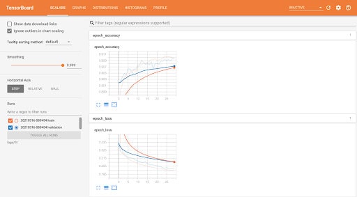
The “Runs” tab on the sidebar shows logs from different runs both for training and validation. Adjustable smoothing scroller helps to smoothen the line charts.
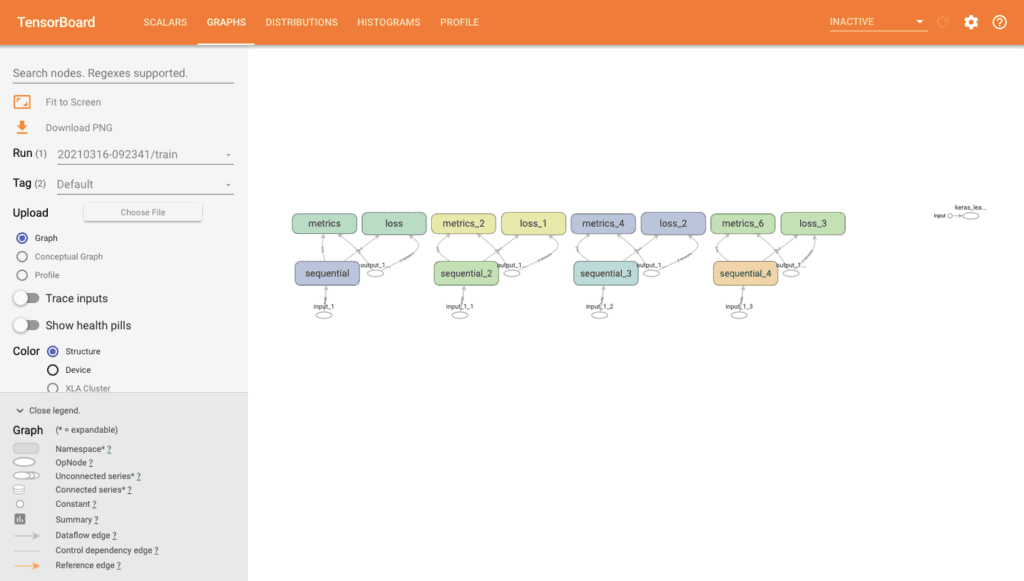
Tensorboard Graphs
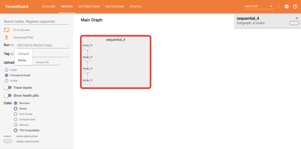
Model graphs show the model’s design and you can easily determine whether it matches your desired design. By default, an op-level graph is selected as “Default” on tags but you can change to “Keras” by selecting it on tags. The op-level graph shows how TensorFlow understood your program and it can be a guide on how to change your model.
If Keras is selected on tags, double click on the sequential node, and you will see its structure. It displays a conceptual graph that shows how Keras views your model. This is useful when you are reusing an already saved model and you are interested in validating its structure.
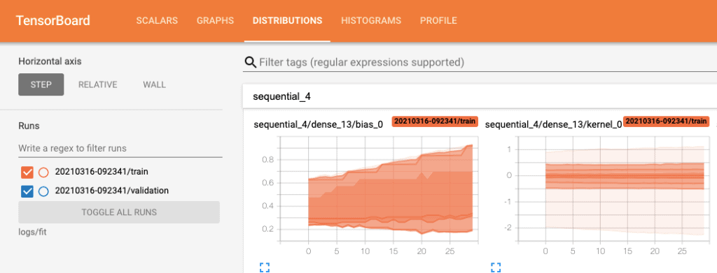
Tensorboard Distribution
This shows the distribution of tensors and it is used for showing the distribution of weights and biases in every epoch- whether they are changing as expected.
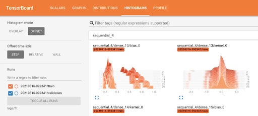
Tensorboard Histograms
This shows the distribution of tensors in histograms and it is used for showing the distribution of weights and biases in every epoch – whether they are changing as expected.
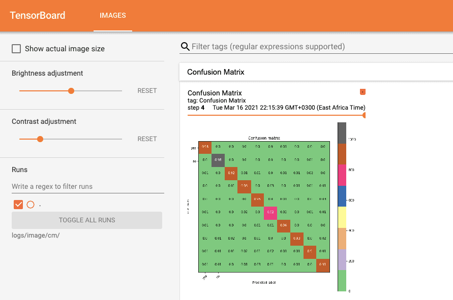
Exploring confusion matrix evolution on TensorBoard
A confusion matrix is a table-like model output showing model performance, each row showing predicted and columns showing actual values. When building a machine learning model, especially when solving a classification problem, a confusion matrix or an error matrix is a very good tool to use.
Tensorboard can help us log the confusion matrix for every epoch, let’s log the confusion matrix using the `mnist` dataset provided by Keras datasets.
First, import necessary libraries and dataset
import numpy as np
import pandas as pd
import tensorflow as tf
import datetime
import sklearn

mnist = tf.keras.datasets.mnist

(X_train, y_train), (X_test, y_test) = mnist.load_data()
X_train, X_test = X_train / 255.0, X_test / 255.0
Define class_names
class_names = ['Zero','One','Two','Three','Four','Five','Six','Seven','Eight','Nine']
Let’s create a function taking advantage of `matplotlib` – python visualization library -, to create a plotted graph with a confusion matrix.
import itertools
import matplotlib.pyplot as plt

def plot_confusion_matrix(cm, class_names):
    figure = plt.figure(figsize=(8, 8))
    plt.imshow(cm, interpolation='nearest', cmap=plt.cm.Accent)
    plt.title("Confusion matrix")
    plt.colorbar()
    tick_marks = np.arange(len(class_names))
    plt.xticks(tick_marks, class_names, rotation=45)
    plt.yticks(tick_marks, class_names)

    cm = np.around(cm.astype('float') / cm.sum(axis=1)[:, np.newaxis], decimals=2)
    threshold = cm.max() / 2.

    for i, j in itertools.product(range(cm.shape[0]), range(cm.shape[1])):
        color = "white" if cm[i, j] > threshold else "black"
        plt.text(j, i, cm[i, j], horizontalalignment="center", color=color)

    plt.tight_layout()
    plt.ylabel('True label')
    plt.xlabel('Predicted label')

    return figure
Next, let’s create a logging directory
logdir = "logs/image/"
tensorboard_callback = tf.keras.callbacks.TensorBoard(log_dir = logdir, histogram_freq = 1)
file_writer_cm = tf.summary.create_file_writer(logdir + '/cm')
Since `matplotlib` file format can’t be converted to an image, we are going to create a function that will convert `matplotlib` to png
def plot_to_image(figure):
buf = io.BytesIO()
plt.savefig(buf, format='png')
plt.close(figure)
buf.seek(0)

digit = tf.image.decode_png(buf.getvalue(), channels=4)
digit = tf.expand_dims(digit, 0)

return digit
Next, the ‘log_confusion_matrix’ function will take advantage of ‘file_writer_cm’ to log our confusion matrix after every epoch.
from tensorflow import keras
from sklearn import metrics
import io

def log_confusion_matrix(epoch, logs):
    predictions = model.predict(X_test)
    predictions = np.argmax(predictions, axis=1)

    cm = metrics.confusion_matrix(y_test, predictions)
    figure = plot_confusion_matrix(cm, class_names=class_names)
    cm_image = plot_to_image(figure)

    with file_writer_cm.as_default():
        tf.summary.image("Confusion Matrix", cm_image, step=epoch)
Create a callback using LambdaCallback while passing our logging function as a parameter. Finally, create a model and fit our model then launch Tensorboard.
cm_callback = tf.keras.callbacks.LambdaCallback(on_epoch_end=log_confusion_matrix)

model = tf.keras.models.Sequential([
   tf.keras.layers.Flatten(input_shape=(28, 28)),
   tf.keras.layers.Dense(512, activation='relu'),
   tf.keras.layers.Dropout(0.2),
   tf.keras.layers.Dense(10, activation='softmax')])

model.compile(optimizer='sgd', loss='sparse_categorical_crossentropy',metrics=['accuracy'])

model.fit(X_train, y_train, batch_size = 32, validation_split=0.2, epochs = 30, callbacks=[tensorboard_callback, cm_callback])
tensorboard --logdir logs/image/cm/
Under the Images tab, you will see the graph showing the confusion matrix, you can adjust the progress bar for every epoch and you can see the confusion matrix at every step.
How to Use the TensorBoard projector
A Tensorboard projector is a graphical tool for representing high-dimensional embeddings, a projector is necessary when you want to visualize images or words as well as understanding your embedding layer.
To use the projector you first have to load it from the Tensorflow plugins module via the code below.
from tensorboard.plugins import projector
How to display image data in TensorBoard
If you want to visualize layer weights, generated tensors or input data, TensorFlow Image Summary API helps you view them on TensorBoard Images.
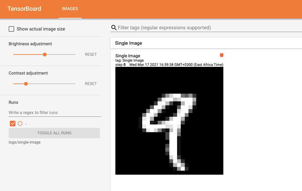
Visualizing a single image in TensorBoard
The shape of a single image in our data set is (28,28) known as a rank-2 tensor, this represents the height and width of the image. You can examine this by running the following code
print(X_train[0].shape)
Since we are going to use `tf.summary.image()` which expects rank-4 tensor, we have to reshape using the `numpy` reshape method. Our output should contain (batch_size, height, width, channels).
Since we are logging a single image and our image is grayscale, we are setting both batch_size and ‘channels’ values as 1.
First, let’s delete old logs and create a file writer.
rm -rf ./logs/
logdir = "logs/single-image/"
file_writer = tf.summary.create_file_writer(logdir)
Next, log the image to TensorBoard
import numpy as np

with file_writer.as_default():
    image = np.reshape(X_train[4], (-1, 28, 28, 1))
    tf.summary.image("Single Image", image, step=0)
Launch tensorboard
tensorboard --logdir logs/single-image
Output
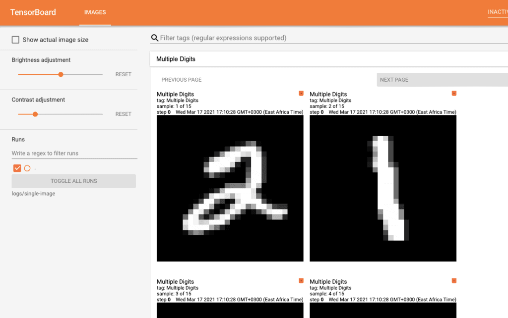
Visualizing multiple images in TensorBoard
You can visualize multiple images, by setting a range as follows:
import numpy as np

with file_writer.as_default():
    images = np.reshape(X_train[5:20], (-1, 28, 28, 1))
    tf.summary.image("Multiple Digits", images, max_outputs=16, step=0)
Visualizing actual images in TensorBoard
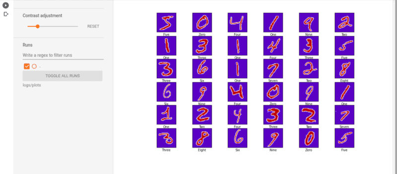
From the above two examples, you have been visualizing mnist tensors. However, using `matplotlib`, you can visualize the actual images by logging them in TensorBoard.
Clear previous logs
rm -rf logs
Import `matplotlib` library and create class names and initiate ‘tf.summary.create_file_writer’.
import io
import matplotlib.pyplot as plt

class_names = ['Zero','One','Two','Three','Four','Five','Six','Seven','Eight','Nine']
logdir = "logs/actual-images/"
file_writer = tf.summary.create_file_writer(logdir)
Write a function that will create grid of mnist images
def image_grid():
figure = plt.figure(figsize=(12,8))

for i in range(25):
    plt.subplot(5, 5, i + 1)
    plt.xlabel(class_names[y_train[i]])
    plt.xticks([])
    plt.yticks([])
    plt.grid(False)
    plt.imshow(X_train[i], cmap=plt.cm.coolwarm)

return figure
Next, let’s write a function that will convert this 5X5 grid into a single image that will be logged in to Tensorboard logs
def plot_to_image(figure):
buf = io.BytesIO()
plt.savefig(buf, format='png')
plt.close(figure)
buf.seek(0)
image = tf.image.decode_png(buf.getvalue(), channels=4)
image = tf.expand_dims(image, 0)
return image
Launch Tensorboard
tensorboard --logdir logs/actual-images
Hyperparameter tuning with TensorBoard
In machine learning, Hyperparemeters are parameters that are useful in controlling the learning process when building our models. Hyperparameters can be classified into two:
- Model hyperparameters – value can’t be estimated from the data because they infer from model selection tasks. Examples include the topology and size of the neural network.
- Algorithm hyperparameters – Affects speed and quality of the learning process but has no influence on how the model performs. Examples include mini-batch size and learning rate.
Choice of hyperparameters like dropout rate in a layer or learning rate affects models accuracy or loss.
Using our `mnist` dataset, let’s demonstrate how to perform hyperparameter tuning using TensorBoard.
Start by clearing previous logs
rm -rf ./logs/
From TensorBoard plugins, let’s import hparam’ api module
from tensorboard.plugins.hparams import api as hp
Create a new log directory
logdir = "logs/hparamas"
Let’s experiment with tuning three hyperparameters which are:
- Number of units in our first layer
- In dropout layer, dropout rate
- Optimizer function
Next, let’s list values that will be used in the example.
HP_NUM_UNITS = hp.HParam('num_units', hp.Discrete([16, 17]))
HP_DROPOUT = hp.HParam('dropout', hp.RealInterval(0.1,0.2))
HP_OPTIMIZER = hp.HParam('optimizer', hp.Discrete(['adam', 'sgd', 'rmsprop']))
Use tf.summary.create_file_writer() method to write to our logs folder.
METRIC_ACCURACY = 'accuracy'

with tf.summary.create_file_writer(logdir).as_default():
    hp.hparams_config(
        hparams=[HP_NUM_UNITS, HP_DROPOUT, HP_OPTIMIZER],
        metrics=[hp.Metric(METRIC_ACCURACY, display_name='Accuracy')],)
If you don’t perform the above step, you can use a string literal instead, i.e hparams[‘dropout’] instead of hparams[HP_DROPOUT]
Now let’s create a function that will take parameters from `hparams` dictionary defined above rather than the hard coding done on previous examples and use them during the training process.
def create_model(hparams):
    model = tf.keras.models.Sequential([
        tf.keras.layers.Flatten(input_shape=(28, 28)),
        tf.keras.layers.Dense(hparams[HP_NUM_UNITS],  activation='relu'),
        tf.keras.layers.Dropout(hparams[HP_DROPOUT]),
        tf.keras.layers.Dense(10, activation='softmax')])

    model.compile(optimizer=hparams[HP_OPTIMIZER],
                  loss='sparse_categorical_crossentropy',
                  metrics=['accuracy'])

    model.fit(X_train, y_train, epochs=5)
    loss, accuracy = model.evaluate(X_test, y_test)

    return accuracy
Next, let’s create a run function that would log a summary of `hparams` with final accuracy and hyperparameters.
def experiment(experiment_dir, hparams):

    with tf.summary.create_file_writer(experiment_dir).as_default():
        hp.hparams(hparams)
        accuracy = create_model(hparams)
        tf.summary.scalar(METRIC_ACCURACY, accuracy, step=1)
Next, start training our model using different sets of hyperparameters, for this example, we are going to try a number of combinations including upper and lower bound of real-valued parameters.
experiment_no = 0

for num_units in HP_NUM_UNITS.domain.values:
    for dropout_rate in (HP_DROPOUT.domain.min_value, HP_DROPOUT.domain.max_value):
        for optimizer in HP_OPTIMIZER.domain.values:
            hparams = {
                HP_NUM_UNITS: num_units,
                HP_DROPOUT: dropout_rate,
                HP_OPTIMIZER: optimizer,}

            experiment_name = f'Experiment {experiment_no}'
            print(f'Starting Experiment: {experiment_name}')
            print({h.name: hparams[h] for h in hparams})
            experiment(logdir + experiment_name, hparams)
            experiment_no += 1
Launch TensorBoard on your browser or on your notebook and click on “HParams” at the top
tensorboard -- logdir logs/hparam_tuning
Note: During this tutorial, you’ll use a few `hparams` for the first training.
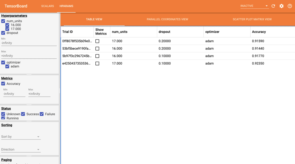
The left panel allows us to filter quite a number of features which include: hyperparameters or metrics, hyperparameters/metrics values to be shown in the dashboard, run status, sort hyperparameters/metric in the table’s view and a number of session groups to display.
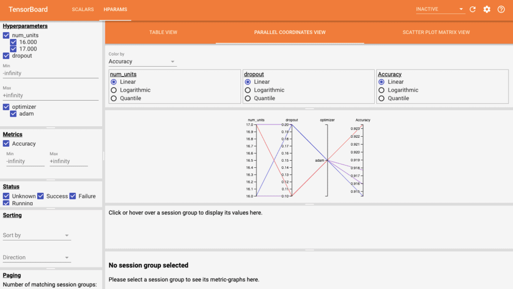
Hparams dashboard has three tabs:
- Table view – shows runs, hyperparameters and metrics
- Parallel Coordinates View – shows every run as a line moving through an axis for each of the hyperparameters and accuracy metric.
- Scatter Plot View – display plots comparing each hyperparameter/metric with each metric.
Profile model performance using TensorFlow Profiler
Machine learning algorithms consume a lot of resources during computation. Therefore, a tool like Tensorflow profiler is crucial for ensuring that you are running the most optimized version of your models.
Setup
Tensorflow profiler requires the latest version of Tensorflow and TensorBoard. Use the below command to install it in your working environment.
pip install -U tensorboard_plugin_profile
The next step is to check whether Tensorflow has access to your device GPU
device_name = tf.test.gpu_device_name()
if not device_name:
 raise SystemError('GPU device not found')
print('Found GPU at: {}'.format(device_name))
If you get a system error that GPU devices can’t be found, kindly consider using Google Colab for this part of the tutorial. Once you have it started, on the runtime tab, click “Change Runtime” and select GPU in options because by default “None” is selected.
Remove previous logs and create a new log directory.
rm -rf ./logs/
logdir = "logs"
Import TensorBoard callback module and create a callback
from tensorflow.keras.callbacks import TensorBoard
callbacks = [TensorBoard(log_dir=logdir, profile_batch='10,20')]
Create our model and compile
model = tf.keras.models.Sequential([
  tf.keras.layers.Flatten(input_shape=(28, 28)),
  tf.keras.layers.Dense(512, activation='relu'),
  tf.keras.layers.Dropout(0.2),
  tf.keras.layers.Dense(10, activation='softmax')])

model.compile(optimizer='sgd', loss='sparse_categorical_crossentropy',metrics=['accuracy'])
Fit training data to model
model.fit(X_train, y_train, epochs=10, validation_split=0.2, callbacks=callbacks)
Load tensorboard to our notebook and launch it
load_ext tensorboard
tensorboard --logdir logs
Output
Once the TensorBoard dashboard is launched, go to the ‘inactive’ tab and select ‘Profile’, you will see the window below. On the left panel, there are a number of drop-down menus, pick the tools menu. This has a number of options/tools, including Overview page (default), input pipeline analyzer, kernel stats, memory profile, pd viewer, TensorFlow stats, Tensorflow data bottleneck analysis and trace viewer.
Overview Page
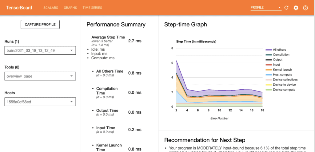
This overview page shows a high-level performance of our model, it has sections which like:
Performance Summary
It shows the average step time for every process, these processes include: All other time, compilations time, output time, input time, kernel launch time and host compute time.
Step--time Graph
This is a graph showing the time it took in every process for every step, If you hover on the topmost layer at every step, you will see time for every process at that specific stage.
Recommendations for Next Step
This section holds recommendations that you can use on the next training so that you can improve the performance of your model during training.
Run Environment
Shows environment where your model is running on, this includes: number of hosts used, device type and number of devices cores
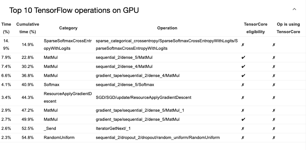
Top 10 TensorFlow operations on GPU
Trace Viewer
In order to understand where the performance bottleneck occurs in the input pipeline, Trace viewer which is under the tools’ dropdown menu shows you when each activity happened on the CPU and GPU during model profiling.
The vertical axis shows various event groups. Each event group has a horizontal timeline of events executed on GPU streams. Events are colored and are in a rectangular block against their own timeline.
You can click on a single event and analyze further its performance.
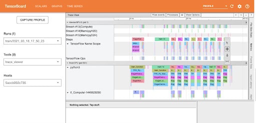
You can also select a number of events at the same time by selecting them while holding the CTRL key or CMD key in mac.
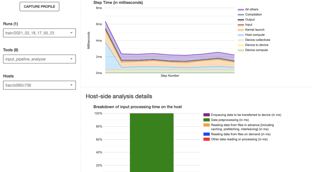
Input pipeline analyzer
Helpful in analyzing the input pipeline and providing recommendations, Analysis is divided into three sections: device side, host side and input operations statistics.
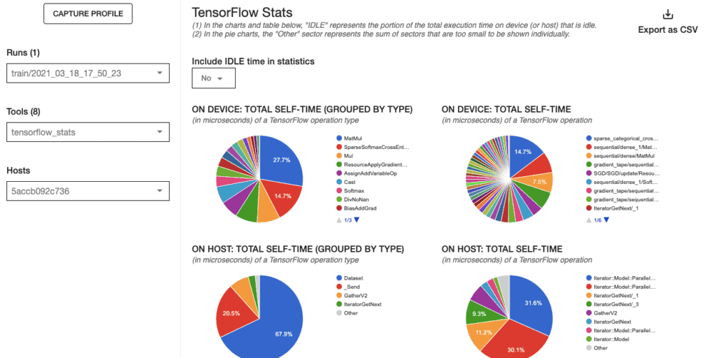
Tensorflow Statistics
It shows Tensorflow’s total execution time for every process on device or host. Select Yes on “Include IDLE time in statistics” to include idle time on the pie charts.
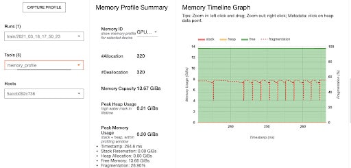
Memory Profile
Provide memory summary, memory timeline graph and memory breakdown table
Using TensorBoard Debugger
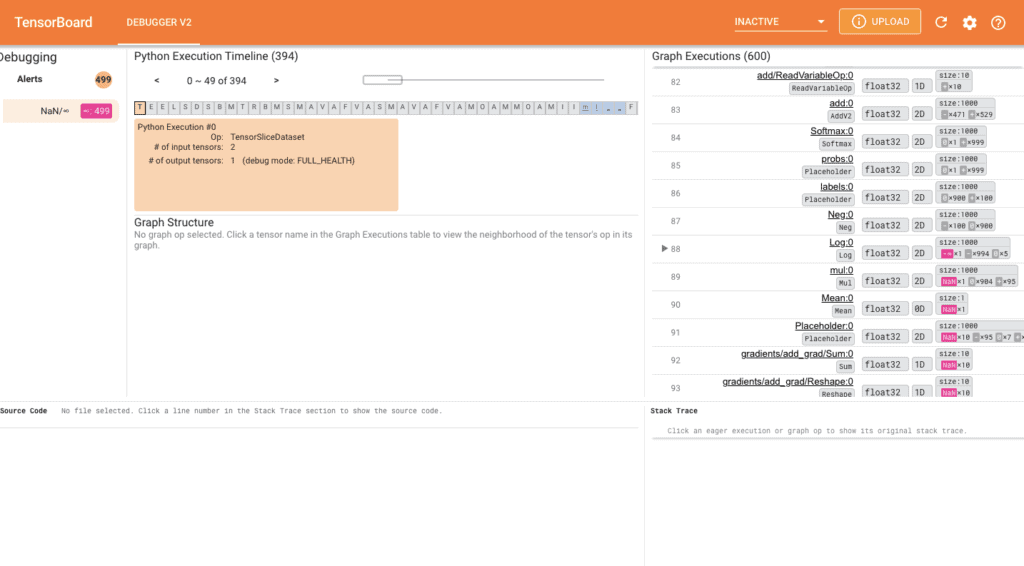
During model training using Tensorflow, events which involve NANs can affect the training process leading to the non-improvement in model accuracy in subsequent steps. TensorBoard 2.3+ (together with TensorFlow 2.3+) provides a debugging tool known as Debugger 2. This tool will help track NANs in a Neural Network written in Tensorflow.
Here’s an example provided in the TensorFlow Github which involves training the mnist dataset and capturing NANs then analyzing our results on TensorBoard debugger 2.
First, Navigate to project root on your terminal and run the below command.
python -m tensorflow.python.debug.examps.v2.debug_mnist_v2 --dump_dir /tmp/tfdbg2_logdir --dump_tensor_debug_mode FULL_HEALTH
Once the above command runs, you will notice non-improvement in model accuracy displayed on the terminal. This is caused by NANs, you can launch a TensorBoard debugger 2 by the following command.
tensorboard --logdir /tmp/tfdbg2_logdir
Output
To invoke the debugger on your model, use tf.debugging.experimental.enable_dump_debug_info() which is the API entry point of Debugger V2. It takes parameters:
- logdir which is log directory
- tensor_debug_mode – controls information debugger extract from each aeger or in-graph tensor
- circular_buffer_size – controls number of tensor events to be saved. Default is 1000 and unsetting it, use value -1
tf.debugging.experimental.enable_dump_debug_info(
  logdir,
  tensor_debug_mode="FULL_HEALTH",
  circular_buffer_size=-1)
Copy
If you don’t have NANs in your model, you will see a blank Debugger 2 on your TensorBoard dashboard.
Using TensorBoard with deep learning frameworks
Since this tutorial has majored on using Tensorflow and Keras with TensorBoard, it doesn’t mean that it can only work with just those. You can also use other machine learning frameworks such as PyTorch, MXNet, CNTK (Microsoft Cognitive Toolkit) and XGBoost, etc.
TensorBoard with XGBoost
from tensorboardX import SummaryWriter

def TensorBoardCallback():
    writer = SummaryWriter()

    def callback(env):
        for k, v in env.evaluation_result_list:
            writer.add_scalar(k, v, env.iteration)

    return callback

xgb.train(callbacks=[TensorBoardCallback()])
TensorBoard with Pytorch
from torch.utils.tensorboard import SummaryWriter

writer = SummaryWriter(log_dir='logs')

from torch.utils.tensorboard import SummaryWriter
import numpy as np

for n_iter in range(100):
    writer.add_scalar('Loss/train', np.random.random(), n_iter)
    writer.add_scalar('Loss/test', np.random.random(), n_iter)
    writer.add_scalar('Accuracy/train', np.random.random(), n_iter)
    writer.add_scalar('Accuracy/test', np.random.random(), n_iter
Tensorboard.dev
Once you have your TensorBoard experiment results ready and you would like to track, host or share them with your team Tensorboard.dev is a go-to tool. Using a few simple commands you will make your project available for your team.
Go to your project folder on your terminal where you have logs already generated, Ensure that the Tensorflow environment with TensorBoard is active.
tensorboard dev upload --logdir logs \
--name "(optional) My latest experiment" \
--description "(optional) Simple comparison of several hyperparameters"
You will get a link, copy it on your browser, once loaded, you will get an authorization key. Enter it and you will get a link to your new TensorBoard Dashboard.
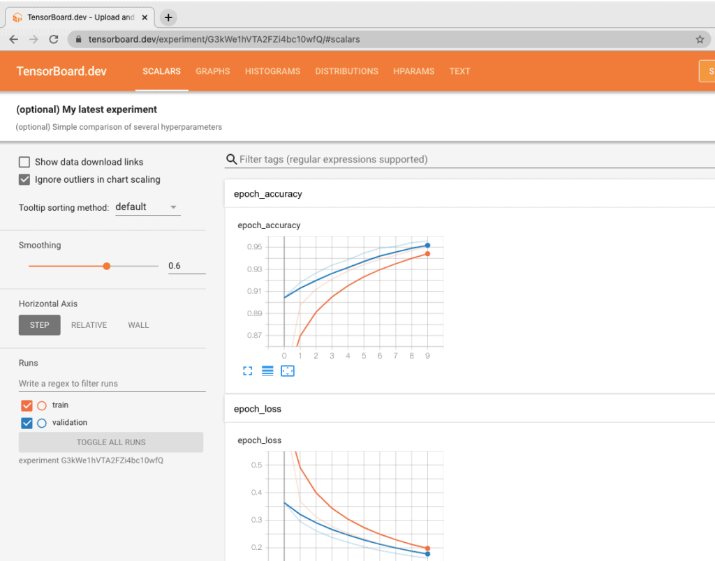
Share it!
Limitations of using TensorBoard
As much as TensorBoard has all those amazing features, there are also quite a number of limitations i.e:
- Difficulty in logging and visualizing audio/visual data.
- Limitations on the number of runs since interface can’t handle them on User Interface.
- Versioning of data and models not possible.
- It’s tedious to use team settings hence limiting collaboration.
Conclusion
After exploring all those features provided by TensorBoard and its limitations, you can see why this is a very important tool for monitoring the performance of your machine learning models. The ease of using and developing with TensorBoard makes it a go-to tool when building machine learning models.
本文内容由网友自发贡献,版权归原作者所有,本站不承担相应法律责任。如您发现有涉嫌抄袭侵权的内容,请联系:hwhale#tublm.com(使用前将#替换为@)