这个Project的目的是利用神经卷积网络(CNN)来分类(classify)常见的交通标志。CNN 在电脑读图领域已经全面超过了传统的机器学习电脑读图的方法(SVC, OpenCV)。大量的数据是深度学习准确性的保证, 在数据不够的情况下也可以人为的对原有数据进行小改动从而来提高识别的准确度。
- 导入必要的软件包(pickle, numpy, cv2, matplotlib, sklearn, tensorflow, Keras)
import pickle
import cv2
import matplotlib.pyplot as plt
import numpy as np
from sklearn.model_selection import train_test_split
from keras.preprocessing.image import ImageDataGenerator
from sklearn.model_selection import train_test_split
import tensorflow as tf
from tensorflow.contrib.layers import flatten
import os
%matplotlib inline
- 数据来源:
和大部分的机器学习的要求一样, CNN需要大量有label的数据,German Traffic Sign Dataset提供了对于这个project的研究并给出结果可用于比较,数据在这里可以下载到。解压后就可以用Python导入了:
training_file = '/Volumes/SSD/traffic-signs-data/train.p'
testing_file = '/Volumes/SSD/traffic-signs-data/test.p'
with open(training_file, mode='rb') as f:
train = pickle.load(f)
with open(testing_file, mode='rb') as f:
test = pickle.load(f)
X_train, y_train = train['features'], train['labels']
X_test, y_test = test['features'], test['labels']
n_train = X_train.shape[0]
n_test = X_test.shape[0]
image_shape = X_train[0].shape
n_classes = len(set(y_train))
print("Number of training examples =", n_train)
print("Number of testing examples =", n_test)
print("Image data shape =", image_shape)
print("Number of classes =", n_classes)
输出:
Number of training examples = 39209
Number of testing examples = 12630
Image data shape = (32, 32, 3)
Number of classes = 43
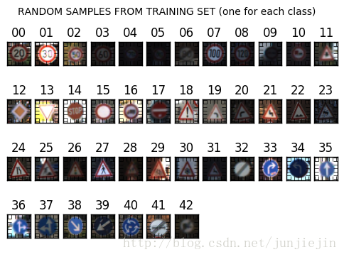
从上面我们可以看到有39209个用作训练的图像 和 12630个testing data。39209张照片对于训练CNN来说是不够的(100000张以上是比较理想的数据量), 所以之后要加入data augment 的模块来人为增加数据。 每张图像的大小是是32x32 并且有3个信道。总共有43个不同的label。
我们也可以把每个label对应的图片随机选择一张画出来。
rows, cols = 4, 12
fig, ax_array = plt.subplots(rows, cols)
plt.suptitle('RANDOM SAMPLES FROM TRAINING SET (one for each class)')
for class_idx, ax in enumerate(ax_array.ravel()):
if class_idx < n_classes:
cur_X = X_train[y_train == class_idx]
cur_img = cur_X[np.random.randint(len(cur_X))]
ax.imshow(cur_img)
ax.set_title('{:02d}'.format(class_idx))
else:
ax.axis('off')
plt.setp([a.get_xticklabels() for a in ax_array.ravel()], visible=False)
plt.setp([a.get_yticklabels() for a in ax_array.ravel()], visible=False)
plt.draw()
我们也可以看看数据的分布情况:
train_distribution, test_distribution = np.zeros(n_classes), np.zeros(n_classes)
for c in range(n_classes):
train_distribution[c] = np.sum(y_train == c) / n_train
test_distribution[c] = np.sum(y_test == c) / n_test
fig, ax = plt.subplots()
col_width = 0.5
bar_train = ax.bar(np.arange(n_classes), train_distribution, width=col_width, color='r')
bar_test = ax.bar(np.arange(n_classes)+col_width, test_distribution, width=col_width, color='b')
ax.set_ylabel('PERCENTAGE OF PRESENCE')
ax.set_xlabel('CLASS LABEL')
ax.set_title('Classes distribution in traffic-sign dataset')
ax.set_xticks(np.arange(0, n_classes, 5) )
ax.set_xticklabels(['{:02d}'.format(c) for c in range(0, n_classes, 5)])
ax.legend((bar_train[0], bar_test[0]), ('train set', 'test set'))
plt.show()
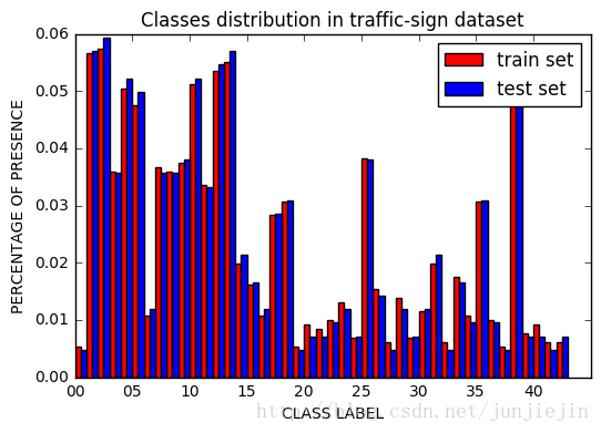
从上图可以看到这42个类别的数据量的分配是很不均匀的。这个会给CNN带来bias(偏见):CNN会更倾向于预测在training data里出现频率多的那些分类。
- 数据前期处理
根据这篇论文[Sermanet, LeCun], 把RGB的照片转化成YUV 然后只选择Y信道的图片可以在不影响精度的同事减少数据计算量。然后每张图片都转化成以0为平均值, 以1为标准差的数组。
def preprocess_features(X, equalize_hist=True):
X = np.array([np.expand_dims(cv2.cvtColor(rgb_img, cv2.COLOR_RGB2YUV)[:, :, 0], 2) for rgb_img in X])
if equalize_hist:
X = np.array([np.expand_dims(cv2.equalizeHist(img), 2) for img in X])
X = np.float32(X)
X -= np.mean(X, axis=0)
X /= (np.std(X, axis=0) + np.finfo('float32').eps)
return X
X_train_norm = preprocess_features(X_train)
X_test_norm = preprocess_features(X_test)
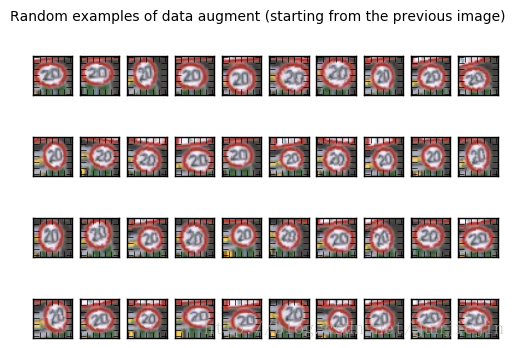
- 人为添加数据(data augment)
对于图片来时, 一定程度的旋转, 上下左右移动, 放大或者缩小都应该不会影响它的标签。 虽然图片数据已经完全不一样了, 我们肉眼还是能够识别的出来, 这能够在增加数据量的同时帮助CNN 总结(generalize). Keras 有个很方便的函数ImageDataGenerator(rotation_range=15.,
zoom_range=0.2,
width_shift_range=0.1,
height_shift_range=0.1) 可以实现这个, 这个函数可以设置 旋转的角度rotation_range, 放大或缩小的倍数zoom_range, 左右移动的比例width_shift_range 和上下移动的比例height_shift_range , 随机在区间内改动原来的照片并产生无数新的照片, 下面我选择一张作为示范:
image_datagen = ImageDataGenerator(rotation_range=15.,
zoom_range=0.2,
width_shift_range=0.1,
height_shift_range=0.1)
img_rgb = X_train[10]
plt.figure(figsize=(1,1))
plt.imshow(img_rgb)
plt.title('Example of RGB image (class = {})'.format(y_train[10]))
plt.axis('off')
plt.show()
rows, cols = 4, 10
fig, ax_array = plt.subplots(rows, cols)
for ax in ax_array.ravel():
augmented_img, _ = image_datagen.flow(np.expand_dims(img_rgb, 0), y_train[10:11]).next()
ax.imshow(np.uint8(np.squeeze(augmented_img)))
plt.setp([a.get_xticklabels() for a in ax_array.ravel()], visible=False)
plt.setp([a.get_yticklabels() for a in ax_array.ravel()], visible=False)
plt.suptitle('Random examples of data augment (starting from the previous image)')
plt.show()
- 搭建CNN
每一层的神经网络都加了dropout 来防止overfitting。这个CNN的特点是把两层conv的output做了一个合成:fc0 = tf.concat([flatten(drop1), flatten(drop2)],1 ) 然后再连接到fully_connected layer 和output layer(42 classes)。文献中说这样做的好处是“the classifier is explicitly provided both the local “motifs” (learned by conv1) and the more “global” shapes and structure (learned by conv2) found in the features.” 我的理解是: CNN 能够在图片的局部和整体都能作为判断的依据,从而提高准确率。
n_classes = 43
def weight_variable(shape, mu=0, sigma=0.1):
initialization = tf.truncated_normal(shape=shape, mean=mu, stddev=sigma)
return tf.Variable(initialization)
def bias_variable(shape, start_val=0.1):
initialization = tf.constant(start_val,shape=shape)
return tf.Variable(initialization)
def conv2d(x, W, strides=[1,1,1,1], padding='SAME'):
return tf.nn.conv2d(input=x, filter=W, strides=strides, padding=padding)
def max_pool2x2(x):
return tf.nn.max_pool(value=x, ksize=[1,2,2,1], strides=[1,2,2,1], padding='SAME')
def my_net(x, n_classes):
c1_out = 64
conv1_W = weight_variable(shape=(3,3,1,c1_out))
conv1_b = bias_variable(shape=(c1_out,))
conv1 = tf.nn.relu(conv2d(x, conv1_W) + conv1_b)
pool1 = max_pool2x2(conv1)
drop1 = tf.nn.dropout(pool1, keep_prob=keep_prob)
c2_out = 128
conv2_W = weight_variable(shape=(3,3,c1_out, c2_out))
conv2_b = bias_variable(shape=(c2_out,))
conv2 = tf.nn.relu(conv2d(drop1, conv2_W) + conv2_b)
pool2 = max_pool2x2(conv2)
drop2 = tf.nn.dropout(pool2, keep_prob=keep_prob)
fc0 = tf.concat([flatten(drop1), flatten(drop2)],1 )
fc1_out = 64
fc1_W = weight_variable(shape=(fc0._shape[1].value, fc1_out))
fc1_b = bias_variable(shape=(fc1_out,))
fc1 = tf.matmul(fc0, fc1_W) + fc1_b
drop_fc1 = tf.nn.dropout(fc1, keep_prob=keep_prob)
fc2_out = n_classes
fc2_W = weight_variable(shape=(drop_fc1._shape[1].value, fc2_out))
fc2_b = bias_variable(shape=(fc2_out,))
logits = tf.matmul(drop_fc1, fc2_W) + fc2_b
return logits
tf.reset_default_graph()
x = tf.placeholder(dtype=tf.float32, shape=(None, 32, 32,1))
y = tf.placeholder(dtype=tf.int64, shape=None)
keep_prob = tf.placeholder(tf.float32)
lr = 0.001
logits = my_net(x, n_classes=n_classes)
cross_entropy = tf.nn.sparse_softmax_cross_entropy_with_logits(logits=logits, labels=y)
loss_function = tf.reduce_mean(cross_entropy)
optimizer = tf.train.AdamOptimizer(learning_rate=lr)
training_operation = optimizer.minimize(loss=loss_function)
correct_prediction = tf.equal(tf.argmax(logits, 1), y)
accuracy_operation = tf.reduce_mean(tf.cast(correct_prediction, tf.float32))
saver = tf.train.Saver()
def evaluate(X_data, y_data):
num_examples = len(X_data)
total_accuracy = 0
sess = tf.get_default_session()
for offset in range(0, num_examples, BATCH_SIZE):
batch_x, batch_y = X_data[offset:offset+BATCH_SIZE], y_data[offset:offset+BATCH_SIZE]
accuracy = sess.run(accuracy_operation, feed_dict={x: batch_x, y: batch_y, keep_prob:1.0})
total_accuracy += (accuracy * len(batch_x))
return total_accuracy / num_examples
EPOCHS = 2
BATCHES_PER_EPOCH = 3
BATCH_SIZE = 128
with tf.Session() as sess:
sess.run(tf.global_variables_initializer())
print("Training...")
print()
for epoch in range(EPOCHS):
batch_counter = 0
for batch_x, batch_y in image_datagen.flow(X_train, y_train, batch_size=BATCH_SIZE):
batch_counter += 1
sess.run(training_operation, feed_dict={x: batch_x, y: batch_y, keep_prob:0.5})
if batch_counter == BATCHES_PER_EPOCH:
break
train_accuracy = evaluate(X_train, y_train)
validation_accuracy = evaluate(X_validation, y_validation)
print("EPOCH {} ...".format(epoch+1))
print("Training Accuracy = {:.3f}, Validation Accuracy = {:.3f}".format(train_accuracy, validation_accuracy))
print()
saver.save(sess, save_path='./checkpoints/traffic_sign_model.ckpt', global_step=epoch)
- Training log:
EPOCH 1 …
Train Accuracy = 0.889 - Validation Accuracy: 0.890
EPOCH 2 …
Train Accuracy = 0.960 - Validation Accuracy: 0.955
EPOCH 3 …
Train Accuracy = 0.975 - Validation Accuracy: 0.969
EPOCH 4 …
Train Accuracy = 0.985 - Validation Accuracy: 0.977
EPOCH 5 …
Train Accuracy = 0.987 - Validation Accuracy: 0.978
EPOCH 6 …
Train Accuracy = 0.991 - Validation Accuracy: 0.985
EPOCH 7 …
Train Accuracy = 0.991 - Validation Accuracy: 0.984
EPOCH 8 …
Train Accuracy = 0.991 - Validation Accuracy: 0.985
EPOCH 9 …
Train Accuracy = 0.991 - Validation Accuracy: 0.985
EPOCH 10 …
Train Accuracy = 0.994 - Validation Accuracy: 0.988
EPOCH 11 …
Train Accuracy = 0.996 - Validation Accuracy: 0.990
EPOCH 12 …
Train Accuracy = 0.995 - Validation Accuracy: 0.989
EPOCH 13 …
Train Accuracy = 0.995 - Validation Accuracy: 0.991
EPOCH 14 …
Train Accuracy = 0.993 - Validation Accuracy: 0.988
EPOCH 15 …
Train Accuracy = 0.995 - Validation Accuracy: 0.989
EPOCH 16 …
Train Accuracy = 0.996 - Validation Accuracy: 0.992
EPOCH 17 …
Train Accuracy = 0.996 - Validation Accuracy: 0.992
EPOCH 18 …
Train Accuracy = 0.997 - Validation Accuracy: 0.992
EPOCH 19 …
Train Accuracy = 0.996 - Validation Accuracy: 0.992
EPOCH 20 …
Train Accuracy = 0.993 - Validation Accuracy: 0.986
EPOCH 21 …
Train Accuracy = 0.997 - Validation Accuracy: 0.993
EPOCH 22 …
Train Accuracy = 0.995 - Validation Accuracy: 0.988
EPOCH 23 …
Train Accuracy = 0.996 - Validation Accuracy: 0.990
EPOCH 24 …
Train Accuracy = 0.996 - Validation Accuracy: 0.991
EPOCH 25 …
Train Accuracy = 0.997 - Validation Accuracy: 0.991
EPOCH 26 …
Train Accuracy = 0.997 - Validation Accuracy: 0.991
EPOCH 27 …
Train Accuracy = 0.996 - Validation Accuracy: 0.994
EPOCH 28 …
Train Accuracy = 0.997 - Validation Accuracy: 0.992
EPOCH 29 …
Train Accuracy = 0.996 - Validation Accuracy: 0.992
EPOCH 30 …
Train Accuracy = 0.996 - Validation Accuracy: 0.991
在EPOCH=27的时候, Validation Accuracy达到了最高 99.4%
可以在测试的时候载入这个模型用来最终 test set 的测试
with tf.Session() as sess:
checkpointer.restore(sess, '../checkpoints/traffic_sign_model.ckpt-27')
test_accuracy = evaluate(X_test_norm, y_test)
print('Performance on test set: {:.3f}'.format(test_accuracy))
>>> Performance on test set: 0.953
在test data set上有95.3% 的准确率!
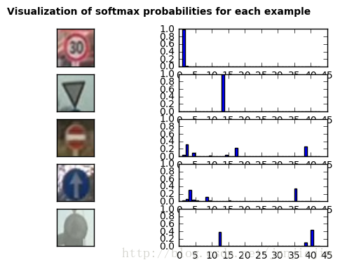
网上找了5张图片来做测试:
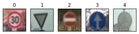
5张图里对了4张。以下是每张图的probability, 从中可以看到CNN预测的confidence:
本文内容由网友自发贡献,版权归原作者所有,本站不承担相应法律责任。如您发现有涉嫌抄袭侵权的内容,请联系:hwhale#tublm.com(使用前将#替换为@)