In [8]: kmeans.fit(scaled_features)Out[8]:KMeans(init='random', n_clusters=3, random_state=42)
使用最低 SSE 运行的初始化统计数据可作为以下属性使用:kmeans打电话后.fit():
>>>
In [9]: # The lowest SSE value ...: kmeans.inertia_Out[9]: 74.57960106819854In [10]: # Final locations of the centroid ...: kmeans.cluster_centers_Out[10]:array([[ 1.19539276, 0.13158148], [-0.25813925, 1.05589975], [-0.91941183, -1.18551732]])In [11]: # The number of iterations required to converge ...: kmeans.n_iter_Out[11]: 6
最后,聚类分配作为一维 NumPy 数组存储在kmeans.labels_。以下是前五个预测标签:
>>>
In [12]: kmeans.labels_[:5]Out[12]: array([0, 1, 2, 2, 2], dtype=int32)
In [13]: kmeans_kwargs={ ...: "init":"random", ...: "n_init":10, ...: "max_iter":300, ...: "random_state":42, ...: } ...: ...: # A list holds the SSE values for each k ...: sse=[] ...: forkinrange(1,11): ...: kmeans=KMeans(n_clusters=k,**kmeans_kwargs) ...: kmeans.fit(scaled_features) ...: sse.append(kmeans.inertia_)
In [17]: # A list holds the silhouette coefficients for each k ...: silhouette_coefficients=[] ...: ...: # Notice you start at 2 clusters for silhouette coefficient ...: forkinrange(2,11): ...: kmeans=KMeans(n_clusters=k,**kmeans_kwargs) ...: kmeans.fit(scaled_features) ...: score=silhouette_score(scaled_features,kmeans.labels_) ...: silhouette_coefficients.append(score)
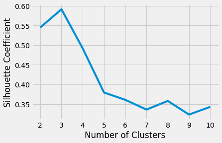
绘制每个的平均轮廓分数k表明最好的选择是k是3因为它有最高分:
>>>
In [18]: plt.style.use("fivethirtyeight") ...: plt.plot(range(2,11),silhouette_coefficients) ...: plt.xticks(range(2,11)) ...: plt.xlabel("Number of Clusters") ...: plt.ylabel("Silhouette Coefficient") ...: plt.show()
In [21]: # Instantiate k-means and dbscan algorithms ...: kmeans=KMeans(n_clusters=2) ...: dbscan=DBSCAN(eps=0.3) ...: ...: # Fit the algorithms to the features ...: kmeans.fit(scaled_features) ...: dbscan.fit(scaled_features) ...: ...: # Compute the silhouette scores for each algorithm ...: kmeans_silhouette=silhouette_score( ...: scaled_features,kmeans.labels_ ...: ).round(2) ...: dbscan_silhouette=silhouette_score( ...: scaled_features,dbscan.labels_ ...: ).round(2)
打印两种算法的轮廓系数并进行比较。轮廓系数越高表明聚类越好,这在这种情况下会产生误导:
>>>
In [22]: kmeans_silhouetteOut[22]: 0.5In [23]: dbscan_silhouetteOut[23]: 0.38
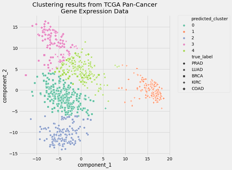
In [2]: uci_tcga_url="https://archive.ics.uci.edu/ml/machine-learning-databases/00401/" ...: archive_name="TCGA-PANCAN-HiSeq-801x20531.tar.gz" ...: # Build the url ...: full_download_url=urllib.parse.urljoin(uci_tcga_url,archive_name) ...: ...: # Download the file ...: r=urllib.request.urlretrieve(full_download_url,archive_name) ...: # Extract the data from the archive ...: tar=tarfile.open(archive_name,"r:gz") ...: tar.extractall() ...: tar.close()
In [21]: # Empty lists to hold evaluation metrics ...: silhouette_scores=[] ...: ari_scores=[] ...: forninrange(2,11): ...: # This set the number of components for pca, ...: # but leaves other steps unchanged ...: pipe["preprocessor"]["pca"].n_components=n ...: pipe.fit(data) ...: ...: silhouette_coef=silhouette_score( ...: pipe["preprocessor"].transform(data), ...: pipe["clusterer"]["kmeans"].labels_, ...: ) ...: ari=adjusted_rand_score( ...: true_labels, ...: pipe["clusterer"]["kmeans"].labels_, ...: ) ...: ...: # Add metrics to their lists ...: silhouette_scores.append(silhouette_coef) ...: ari_scores.append(ari)