作者主页(文火冰糖的硅基工坊):文火冰糖(王文兵)的博客_文火冰糖的硅基工坊_CSDN博客
本文网址:https://blog.csdn.net/HiWangWenBing/article/details/121526014
目录
第1章 概述
1.1 业务需求概述
1.2 业务分析
1.3 导入库
第1章 数据集
1.1 数据集概述
1.2 从文件中读取数据
1.3 提取有效数据
第2章 全连接网络的拟合
2.1 定义全连接网络
2.2 定义loss与优化器
2.3 训练前准备
2.4 开始训练
2.5 loss显示
2.6 结果分析
第3章 RNN网络的拟合
3.1 定义RNN网络
3.2 生成网络
3.3 定义loss与优化器
3.4 训练前的准备
3.5 开始训练
3.6 显示loss
3.7 分析
第1章 概述
1.1 业务需求概述
有一批最近52周的销售数据,希望能够根据这些数据,预测未来几周销售数据。
1.2 业务分析
这是一个线性拟合的问题,那么每周的数据之间是独立的?还是每周的数据之间有时间的相关性?
本文就采用层数的全连接网络和RNN网络对数据进行拟合与比较。
如果全连接网络的拟合度比RNN网络好,则证明每周的数据是独立无关的。
如果全连接网络的拟合度没有RNN网络好,则证明每周的数据是具有时间相关性。
1.3 导入库
%matplotlib inline
import torch
import torch.nn as nn
from torch.nn import functional as F
from torch.autograd import Variable
from torch import optim

import numpy as np
import math, random
import matplotlib.pyplot as plt
import pandas as pd

from torch.utils.data import Dataset
from torch.utils.data import DataLoader
第1章 数据集
1.1 数据集概述
销售数据是通过Excel存放的:包含多个样本数据,每个样本包含52周的数据,如下图所示:
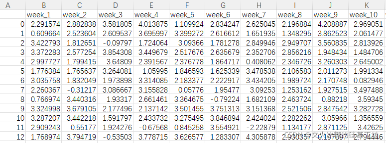
横轴:不同的样本
纵轴:每个样本包含的序列52周的销售数据。
1.2 从文件中读取数据
# 从excel文件中数据
sales_data = pd.read_csv('time_serise_sale.csv')

sales_data.head()
1.3 提取有效数据
# 提取有效数据
source_data = sales_data
source_data.values.shape
source_data.values
array([[0.00000000e+00, 2.29157429e+00, 2.88283833e+00, ...,
        2.52078778e+00, 2.63721001e+00, 2.74892268e+00],
       [1.00000000e+00, 6.09664112e-01, 2.52360427e+00, ...,
        1.66285479e+00, 2.48192522e+00, 2.41120153e+00],
       [2.00000000e+00, 3.42279275e+00, 1.81265116e+00, ...,
        1.72005177e+00, 2.16993942e+00, 2.16170153e+00],
       ...,
       [1.50490000e+04, 3.83370716e+00, 3.54807088e+00, ...,
        3.03134190e+00, 1.85208859e+00, 3.00563077e+00],
       [1.50500000e+04, 3.18643937e+00, 1.70323164e+00, ...,
        1.19605309e+00, 3.34099104e+00, 2.92155740e+00],
       [1.50510000e+04, 3.10427003e+00, 2.82717086e+00, ...,
        1.33781619e+00, 2.71468770e+00, 2.34349413e+00]])
# 显示数据集数据
source_data
| Unnamed: 0 |
week_1 |
week_2 |
week_3 |
week_4 |
week_5 |
week_6 |
week_7 |
week_8 |
week_9 |
... |
week_43 |
week_44 |
week_45 |
week_46 |
week_47 |
week_48 |
week_49 |
week_50 |
week_51 |
week_52 |
| 0 |
0 |
2.291574 |
2.882838 |
3.581805 |
4.013875 |
1.109924 |
2.834247 |
2.625045 |
2.196884 |
4.208887 |
... |
1.242250 |
2.771072 |
3.778143 |
3.161634 |
3.792645 |
2.015481 |
2.826184 |
2.520788 |
2.637210 |
2.748923 |
| 1 |
1 |
0.609664 |
2.523604 |
2.609537 |
3.695997 |
3.399272 |
2.616612 |
1.651935 |
1.348295 |
3.862523 |
... |
2.477505 |
2.284513 |
3.461783 |
3.101052 |
3.442420 |
1.915776 |
2.426168 |
1.662855 |
2.481925 |
2.411202 |
| 2 |
2 |
3.422793 |
1.812651 |
-0.097966 |
1.724064 |
3.093660 |
1.781278 |
2.849946 |
2.949707 |
3.560835 |
... |
2.219667 |
2.359834 |
1.932029 |
2.731947 |
1.836245 |
1.219933 |
1.222740 |
1.720052 |
2.169939 |
2.161702 |
| 3 |
3 |
3.372283 |
2.577254 |
3.854308 |
3.449679 |
2.517676 |
2.635679 |
2.352706 |
2.856216 |
1.948434 |
... |
1.670912 |
0.909113 |
3.216652 |
1.775346 |
3.270484 |
2.399709 |
3.032071 |
1.703666 |
1.750585 |
1.821736 |
| 4 |
4 |
2.997727 |
1.799415 |
3.648090 |
2.391567 |
2.376778 |
1.864717 |
0.408062 |
2.346726 |
3.260303 |
... |
2.304058 |
3.038905 |
2.038733 |
2.825186 |
2.232937 |
2.509050 |
2.881796 |
-1.712131 |
2.140366 |
1.926818 |
| ... |
... |
... |
... |
... |
... |
... |
... |
... |
... |
... |
... |
... |
... |
... |
... |
... |
... |
... |
... |
... |
... |
| 15047 |
15047 |
1.952726 |
1.547637 |
1.902789 |
0.813261 |
2.600979 |
2.910638 |
2.878396 |
0.594216 |
3.526187 |
... |
0.486073 |
3.336252 |
3.307270 |
3.026835 |
1.472116 |
3.220792 |
2.664044 |
1.546153 |
3.026948 |
2.611774 |
| 15048 |
15048 |
0.652824 |
3.589191 |
3.257707 |
2.821276 |
2.185937 |
2.534801 |
-0.774375 |
3.835695 |
3.776809 |
... |
2.684153 |
1.384912 |
3.184570 |
2.832941 |
2.092033 |
2.606198 |
0.753193 |
3.160599 |
3.085800 |
2.814394 |
| 15049 |
15049 |
3.833707 |
3.548071 |
3.194160 |
1.993437 |
3.013547 |
1.825047 |
2.305196 |
0.522475 |
3.126647 |
... |
2.928937 |
1.633754 |
3.078598 |
2.466563 |
0.489380 |
3.518725 |
3.406466 |
3.031342 |
1.852089 |
3.005631 |
| 15050 |
15050 |
3.186439 |
1.703232 |
3.196591 |
2.407803 |
-0.474370 |
3.879943 |
3.762408 |
3.415669 |
1.790529 |
... |
1.642612 |
2.387770 |
2.149893 |
0.688463 |
3.150805 |
3.242209 |
2.972728 |
1.196053 |
3.340991 |
2.921557 |
| 15051 |
15051 |
3.104270 |
2.827171 |
1.176428 |
3.274967 |
2.934655 |
2.349188 |
2.412935 |
1.219054 |
2.843297 |
... |
2.551259 |
0.819203 |
3.416532 |
3.242021 |
2.810177 |
2.037487 |
2.681694 |
1.337816 |
2.714688 |
2.343494 |
15052 rows × 53 columns
第2章 全连接网络的拟合
2.1 定义全连接网络
class FullyConnected(nn.Module):
    def __init__(self, x_size, hidden_size, output_size):
        super(FullyConnected, self).__init__()
        self.hidden_size = hidden_size

        self.linear_with_tanh = nn.Sequential(
            nn.Linear(10, self.hidden_size),
            nn.Tanh(),
            nn.Linear(self.hidden_size, self.hidden_size),
            nn.Tanh(),
            nn.Linear(self.hidden_size, output_size)
        )

    def forward(self, x):
        yhat = self.linear_with_tanh(x)

        return yhat
# 输入样本的size
x_size = 1

# 隐藏层的size:try to change this parameters
hidden_size = 2

#数据特征的size
output_size = 10

fc_model = FullyConnected(x_size = x_size, hidden_size = hidden_size, output_size = output_size)
print(fc_model)

fc_model = fc_model.double()
print(fc_model)
FullyConnected(
  (linear_with_tanh): Sequential(
    (0): Linear(in_features=10, out_features=2, bias=True)
    (1): Tanh()
    (2): Linear(in_features=2, out_features=2, bias=True)
    (3): Tanh()
    (4): Linear(in_features=2, out_features=10, bias=True)
  )
)
fc_model.state_dict()['linear_with_tanh.0.weight']
tensor([[ 0.2028,  0.0721,  0.0101,  0.2866, -0.3106,  0.1612,  0.0082, -0.1394,
          0.2630, -0.2903],
        [ 0.0596, -0.2646,  0.2036, -0.2676, -0.0198,  0.2969,  0.2596,  0.0965,
          0.0746, -0.0195]], dtype=torch.float64)
2.2 定义loss与优化器
#定义loss函数
criterion = nn.MSELoss()

# 使用 Adam 优化器 比课上使用的 SGD 优化器更加稳定
optimizer = optim.AdamW(fc_model.parameters(), lr=0.01)
2.3 训练前准备
n_epochs = 30
n_layers = 1
batch_size = seq_length
seq_length = 10

fc_losses = np.zeros(n_epochs)


data_loader = torch.utils.data.DataLoader(source_data.values, batch_size = batch_size, shuffle=True)
print(data_loader)
print(data_loader.batch_size )
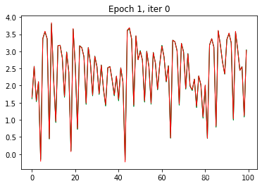
2.4 开始训练
# 开始训练
for epoch in range(n_epochs):
    # 定义用于每个epoch的平均loss
    epoch_losses = []

    # 读取batch数据
    for iter_, data in enumerate(data_loader):
        #当读到数据不足batch size时,跳过batch size
        if data.shape[0] != batch_size:
            continue

        #随机的获取长度=seq_length的数据
        random_index = random.randint(0, data.shape[-1] - seq_length - 1)
        train_x = data[:, random_index: random_index+seq_length]
        #train_y = data[:, random_index + 1: random_index + seq_length + 1]
        train_y = train_x

        #进行前向运算
        outputs = fc_model(train_x.double())

        #复位梯度
        optimizer.zero_grad()

        #求此次前向运算的loss
        loss = criterion(outputs, train_y)

        #反向求导
        loss.backward()

        #梯度迭代
        optimizer.step()

        #
        epoch_losses.append(loss.detach())

        if iter_  == 0:
            plt.clf();
            plt.ion()
            plt.title("Epoch {}, iter {}".format(epoch, iter_))
            plt.plot(torch.flatten(train_y),'c-',linewidth=1,label='Label')
            #plt.plot(torch.flatten(train_x),'g-',linewidth=1,label='Input')
            plt.plot(torch.flatten(outputs.detach()),'r-',linewidth=1,label='Output')
            plt.draw();
            plt.pause(0.05);
    fc_losses[epoch] = np.mean(epoch_losses)

................................................................
2.5 loss显示
plt.plot(fc_losses)
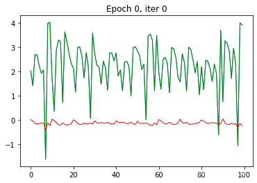
2.6 结果分析
全连接网络应对这种时序序列问题,拟合性不是很好。
第3章 RNN网络的拟合
3.1 定义RNN网络
class SimpleRNN(nn.Module):
    def __init__(self, x_size, hidden_size, n_layers, batch_size, output_size):
        super(SimpleRNN, self).__init__()
        self.hidden_size = hidden_size
        self.n_layers = n_layers
        self.batch_size = batch_size
        #self.inp = nn.Linear(1, hidden_size)
        self.rnn = nn.RNN(x_size, hidden_size, n_layers, batch_first=True)
        self.out = nn.Linear(hidden_size, output_size) # 10 in and 10 out

    def forward(self, inputs, hidden=None):
        hidden = self.__init__hidden()
        #print("Forward hidden {}".format(hidden.shape))
        #print("Forward inps {}".format(inputs.shape))
        output, hidden = self.rnn(inputs.float(), hidden.float())
        #print("Out1 {}".format(output.shape))
        output = self.out(output.float());
        #print("Forward outputs {}".format(output.shape))

        return output, hidden

    def __init__hidden(self):
        hidden = torch.zeros(self.n_layers, self.batch_size, self.hidden_size, dtype=torch.float64)
        return hidden
3.2 生成网络
x_size = 1
hidden_size = 2 # try to change this parameters
n_layers = 1
seq_length = 10
output_size = 1

#rnn_model = SimpleRNN(x_size, hidden_size, n_layers, seq_length, output_size)
rnn_model = SimpleRNN(x_size, hidden_size, n_layers, seq_length, output_size)

print(rnn_model)
SimpleRNN(
  (rnn): RNN(1, 2, batch_first=True)
  (out): Linear(in_features=2, out_features=1, bias=True)
)
3.3 定义loss与优化器
# 定义loss
criterion = nn.MSELoss()

#定义优化器
optimizer = optim.AdamW(rnn_model.parameters(), lr=0.01) # 使用 Adam 优化器 比课上使用的 SGD 优化器更加稳定
3.4 训练前的准备
# 训练前的准备
n_epochs = 30
rnn_losses = np.zeros(n_epochs)

data_loader = torch.utils.data.DataLoader(source_data.values, batch_size=seq_length, shuffle=True)
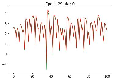
3.5 开始训练
# 开始训练
for epoch in range(n_epochs):
    for iter_, t in enumerate(data_loader):
        if t.shape[0] != seq_length: continue

        random_index = random.randint(0, t.shape[-1] - seq_length - 1)
        train_x = t[:, random_index: random_index+seq_length]
        #train_y = t[:, random_index + 1: random_index + seq_length + 1]
        train_y = train_x

        #获取输出
        outputs, hidden = rnn_model(train_x.double().unsqueeze(2), hidden_size)

        #梯度复位
        optimizer.zero_grad()

        #定义损失函数
        loss = criterion(outputs.double(), train_y.double().unsqueeze(2))

        # 反向求导
        loss.backward()

        #梯度迭代
        optimizer.step()

        #记录loss
        epoch_losses.append(loss.detach())

        #显示拟合图像
        if iter_ == 0:
            plt.clf();
            plt.ion()
            plt.title("Epoch {}, iter {}".format(epoch, iter_))
            plt.plot(torch.flatten(train_y),'c-',linewidth=1,label='Label')
            plt.plot(torch.flatten(train_x),'g-',linewidth=1,label='Input')
            plt.plot(torch.flatten(outputs.detach()),'r-',linewidth=1,label='Output')
            plt.draw();
            plt.pause(0.05);
    rnn_losses[epoch] = np.mean(epoch_losses)
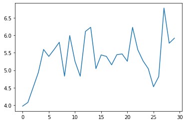
3.6 显示loss
3.7 分析
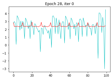
RNN网络在第一个epoch完成后,拟合度就非常好。
作者主页(文火冰糖的硅基工坊):文火冰糖(王文兵)的博客_文火冰糖的硅基工坊_CSDN博客
本文网址:https://blog.csdn.net/HiWangWenBing/article/details/121526014