麦克内马尔检验(McNemar’s Test)
配对标称数据的麦克内马尔检验(McNemar’s Test)
from mlxtend.evaluate import mcnemar
概述
McNemar的检验[1](有时也称为“受试者内卡方检验”)是对配对名义数据的统计检验。在机器学习中,我们可以使用两种统计模型(NEMAR)来测试机器学习的准确性。麦克内马尔的测试是基于两个模型预测的2倍连续表。
McNemar’s Test Statistic
在麦克内马尔的检验中,我们提出了零假设,即概率
p
(
b
)
p(b)
p(b) and
p
(
c
)
p(c)
p(c),或者用简化的术语来说:两个模型中没有一个比另一个更好。因此,另一种假设是,这两种模型的性能并不相同。

McNemar检验统计量(“卡方”)可计算如下:
χ
2
=
(
b
−
c
)
2
(
b
+
c
)
,
\chi^2 = \frac{(b - c)^2}{(b + c)},
χ2=(b+c)(b−c)2,
如果单元格c和b的总和足够大,则
χ
2
\chi^2
χ2 值遵循一个自由度的卡方分布。设置显著性阈值后,例如,
α
=
0.05
α=0.05
α=0.05。我们可以计算
p
p
p 值——假设零假设为真,
p
p
p 值是观察这个经验(或更大)卡方值的概率。如果
p
p
p 值低于我们选择的显著性水平,我们可以拒绝两个模型性能相等的无效假设。
连续性校正
在Quinn McNemar发表McNemar测试[1]大约一年后,Edwards[2]提出了一个连续性修正版本,这是当今更常用的变体:
χ
2
=
(
∣
b
−
c
∣
−
1
)
2
(
b
+
c
)
.
\chi^2 = \frac{( \mid b - c \mid - 1)^2}{(b + c)}.
χ2=(b+c)(∣b−c∣−1)2.
精确p值
如前所述,建议对小样本量(
b
+
c
<
25
b + c < 25
b+c<25[3])进行精确二项检验,因为卡方分布可能无法很好地近似卡方值。精确的p值可计算如下:
p
=
2
∑
i
=
b
n
(
n
i
)
0.
5
i
(
1
−
0.5
)
n
−
i
,
p = 2 \sum^{n}_{i=b} \binom{n}{i} 0.5^i (1 - 0.5)^{n-i},
p=2i=b∑n(in)0.5i(1−0.5)n−i,
其中
n
=
b
+
c
n = b + c
n=b+c,系数2用于计算双边
p
p
p 值。
实例
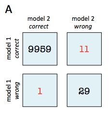
例如,鉴于两个模型的精度分别为99.7%和99.6%,2x2连续性表可以为模型选择提供进一步的见解。

在子图A和B中,两个模型的预测精度如下所示:
- model 1 accuracy: 9,960 / 10,000 = 99.6%
- model 2 accuracy: 9,970 / 10,000 = 99.7%
现在,在子图A中,我们可以看到模型2得到了11个正确的预测,而模型1得到了错误的预测。反之亦然,模型2的预测是对的,模型2的预测是错的。因此,基于这一11:1的比例,我们可以得出结论,模型2的表现明显优于模型1。然而,在子图B中,比例为25:15,这对于选择哪种模型更好来说不太确定。
在下面的编码示例中,我们将使用这两种场景A和B来说明McNemar的测试。
References
示例1-创建2x2连续表
mcnemar功能需要2x2列联表作为NumPy数组,格式如下:

可以使用mlxtend的mcnemar_表函数创建这样的邻接矩阵。估计例如:
import numpy as np
from mlxtend.evaluate import mcnemar_table

# The correct target (class) labels
y_target = np.array([0, 0, 0, 0, 0, 1, 1, 1, 1, 1])

# Class labels predicted by model 1
y_model1 = np.array([0, 1, 0, 0, 0, 1, 1, 0, 0, 0])

# Class labels predicted by model 2
y_model2 = np.array([0, 0, 1, 1, 0, 1, 1, 0, 0, 0])

tb = mcnemar_table(y_target=y_target,
                   y_model1=y_model1,
                   y_model2=y_model2)

print(tb)
[[4 1]
 [2 3]]
示例2——麦克内马尔对方案B的测试
不,让我们继续概述部分中提到的示例,并假设我们已经计算了2x2连续表:

import numpy as np

tb_b = np.array([[9945, 25],
                 [15, 15]])
为了检验两个模型的预测性能相等的零假设(使用显著性水平
α
=
0.05
α=0.05
α=0.05 ),我们可以进行修正的麦克内马尔检验,以计算卡方( chi-squared )和 p值(p-value),如下所示:
from mlxtend.evaluate import mcnemar

chi2, p = mcnemar(ary=tb_b, corrected=True)
print('chi-squared:', chi2)
print('p-value:', p)
chi-squared: 2.025
p-value: 0.154728923485
由于
p
p
p 值大于我们假设的显著性阈值(
α
=
0.05
α=0.05
α=0.05),我们不能拒绝我们的零假设,并假设两个预测模型之间没有显著差异。
示例3——麦克内马尔对场景A的测试
与方案B(例2)相比,方案A中的样本量相对较小(
b
+
c
=
11
+
1
=
12
b+c=11+1=12
b+c=11+1=12),且小于建议的25[3],以通过卡方分布井近似计算出的卡方值。
在这种情况下,我们需要根据二项分布计算精确的p值:
from mlxtend.evaluate import mcnemar
import numpy as np

tb_a = np.array([[9959, 11],
                 [1, 29]])

chi2, p = mcnemar(ary=tb_a, exact=True)

print('chi-squared:', chi2)
print('p-value:', p)
chi-squared: None
p-value: 0.005859375
假设我们在显著性水平
α
=
0.05
α=0.05
α=0.05 的情况下进行了该测试,我们可以拒绝两个模型在该数据集上表现相同的无效假设,因为
p
p
p 值(p≈0.006)小于
α
α
α。
API
mcnemar(ary, corrected=True, exact=False)
配对标称数据的McNemar检验
参数
-
ary : array-like, shape=[2, 2]
2 x 2 contigency table (as returned by evaluate.mcnemar_table), where a: ary[0, 0]: # of samples that both models predicted correctly b: ary[0, 1]: # of samples that model 1 got right and model 2 got wrong c: ary[1, 0]: # of samples that model 2 got right and model 1 got wrong d: aryCell [1, 1]: # of samples that both models predicted incorrectly
2 x 2 contigency table(由evaluate.mcnemar_table返回),
其中
- a:ary[0,0]:# 两个模型正确预测的样本
- b:ary[0,1]:#模型1正确预测的样本和模型2错误预测的样本
- c:ary[1,0]:#模型2正确预测的样本和模型1错误预测的样本
- d:aryCell[1,1]:#两个模型都预测错误的样本数量
-
corrected : array-like, shape=[n_samples] (default: True)
如果True,则使用Edward的连续性校正进行卡方检验
-
exact : bool, (default: False)
If True, uses an exact binomial test comparing b to a binomial distribution with n = b + c and p = 0.5. It is highly recommended to use exact=True for sample sizes < 25 since chi-squared is not well-approximated by the chi-squared distribution!
如果 True,则使用精确的二项检验,将 b 与 n=b+c 且 p=0.5 的二项分布进行比较。对于小于25的样本量,强烈建议使用’exact=True’,因为卡方分布不能很好地近似卡方分布!
Returns
-
chi2, p : float or None, float
返回卡方值和p值;如果’exact=True’(默认值为’False’),‘chi2’是’None’`
Examples
For usage examples, please see
[http://rasbt.github.io/mlxtend/user_guide/evaluate/mcnemar/](http://rasbt.github.io/mlxtend/user_guide/evaluate/mcnemar/)
reference
@online{Raschka2021Sep,
author = {Raschka, S.},
title = {{McNemar’s Test - mlxtend}},
year = {2021},
month = {9},
date = {2021-09-03},
urldate = {2022-03-10},
language = {english},
hyphenation = {english},
note = {[Online; accessed 10. Mar. 2022]},
url = {http://rasbt.github.io/mlxtend/user_guide/evaluate/mcnemar},
abstract = {{A library consisting of useful tools and extensions for the day-to-day data science tasks.}}
}