【OpenCV图像处理】1.18 拉普拉斯算子 - Laplance算子

1. 相关理论

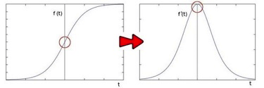
在上一节已经提到过， f ( t ) f(t) f(t)的一阶导就是 f ′ ( t ) f'(t) f′(t)，对应的是Sobel算子，二阶导就是 f ′ ′ ( t ) f''(t) f′′(t)，对应的就是本节的拉普拉斯算子。对应的图形如下所示：

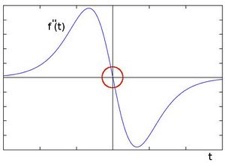
针对上图的解释：在二阶导数的时候，最大变化处的值为零即边缘是零值。通过二阶导数计算，依据此理论我们可以计算图像二阶导数，提取边缘。

• Laplance算子

  • 如果二阶导数不会，别担心 -->拉普拉斯算子(Laplance operator)
    Laplace ( f ) = ∂ 2 f ∂ x 2 + ∂ 2 f ∂ y 2 \text {Laplace}(f)=\frac{\partial^{2} f}{\partial x^{2}}+\frac{\partial^{2} f}{\partial y^{2}} Laplace(f)=∂x2∂2f​+∂y2∂2f​
  • Opencv已经提供了相关API - cv::Laplance

• 处理流程

  • 高斯模糊 – 去噪声GaussianBlur()
  • 转换为灰度图像cvtColor()
  • 拉普拉斯 – 二阶导数计算Laplacian()
  • 取绝对值convertScaleAbs()
  • 显示结果

• API使用 - Laplacian

  Laplacian(
  InputArray src,
  OutputArray dst,
  int depth, //深度CV_16S
  int ksize = 1, // 3
  double scale = 1,
  double delta =0.0,
  int borderType = 4
  )
  

2. 代码 & 运行效果

完整代码：

```c
#include <iostream>
#include <string>
#include <opencv2/opencv.hpp>
#include <opencv2/imgproc/types_c.h>

using namespace std;
using namespace cv;

#ifndef P18
#define P18 18
#endif

int main() {
    std::string path = "../fei.JPG";
    cv::Mat img = cv::imread(path, 5);

    string str_input = "input image";
    string str_output = "output image";

    if(img.empty())
    {
        std::cout << "open file failed" << std::endl;
        return -1;
    }
    
#if P18     //拉普拉斯算子
    Mat gray;
    GaussianBlur(img, img,Size(3,3),0,0);
    cvtColor(img,gray, COLOR_BGR2GRAY);

    Mat edge_image;
    Laplacian(gray, edge_image, CV_16S, 3);
    convertScaleAbs(edge_image,edge_image);

    threshold(edge_image, edge_image, 0, 255, THRESH_OTSU | THRESH_BINARY);
    namedWindow("Laplacian",WINDOW_AUTOSIZE);
    imshow("Laplacian",edge_image);
#endif

    cv::waitKey(0);
    cv::destroyAllWindows();
    return 0;
}

代码说明：
threshold函数是图像的阈值操作，具体可见【OpenCV图像处理】1.14 基本阈值操作

运行效果：

第二幅图形，经过拉普拉斯算子运算后的结果和Sobel算子运算结果的差异不太大，Sobel算子的结果为：

这里为什么会有两个不同个结果，是因为不同的处理方法导致的，详细可以参考：【OpenCV图像处理】1.17 Sobel算子