4.3 嵌入法
请参考《数据准备和特征工程》中的相关章节,调试如下代码。

基础知识
import pandas as pd
from sklearn.model_selection import train_test_split
from sklearn.preprocessing import StandardScaler
from sklearn.feature_selection import SelectFromModel
from sklearn.linear_model import LogisticRegression

# 划分训练集和测试集
df_wine = pd.read_csv("data/data20527/wine_data.csv")
X, y = df_wine.iloc[:, 1:], df_wine.iloc[:, 0].values
X_train, X_test, y_train, y_test = train_test_split(
        X, y, test_size=0.3,
        random_state=0,
        stratify=y)

# 特征标准化变换
std = StandardScaler()
X_train_std = std.fit_transform(X_train)
X_test_std = std.fit_transform(X_test)

# 创建对数概率回归模型lr,采取L1惩罚——这是实现嵌入法的关键
lr = LogisticRegression(C=1.0, penalty='l1',solver='liblinear')

# 创建特征选择实例,并规定选择特征的阈值threshold:特征权重的中位数median。
model = SelectFromModel(lr, threshold='median')
X_new = model.fit_transform(X_train_std, y_train)
X_new.shape
(124, 7)
X_train_std.shape
(124, 13)
项目案例
data = pd.read_csv("data/data20533/diabetes.csv")
print(data.shape)

print(data.columns)
(768, 9)
Index(['Pregnancies', 'Glucose', 'BloodPressure', 'SkinThickness', 'Insulin',
       'BMI', 'DiabetesPedigreeFunction', 'Age', 'Outcome'],
      dtype='object')
# !mkdir /home/aistudio/external-libraries
# !pip install -i https://pypi.tuna.tsinghua.edu.cn/simple xgboost -t /home/aistudio/external-libraries
import sys
sys.path.append('/home/aistudio/external-libraries')
X = data.loc[:, :"Age"]
y = data.loc[:, "Outcome":]
# 创建数据模型并训练,xgboost:分布式梯度增强库
from xgboost import XGBClassifier
model = XGBClassifier(eval_metric='mlogloss')
model.fit(X,y)
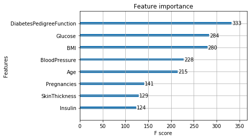
# 训练之后,得到各个特征的重要度,以便进行特征选择
model.feature_importances_
array([0.10621197, 0.2424023 , 0.08803366, 0.07818192, 0.10381887,
       0.1486732 , 0.10059207, 0.13208601], dtype=float32)
%matplotlib inline
from xgboost import plot_importance

plot_importance(model)
selection = SelectFromModel(model, threshold='median', prefit=True)

X_new = selection.transform(X)
X_new.shape, X.shape
((768, 4), (768, 8))
import numpy as np
from sklearn.model_selection import train_test_split
from sklearn.metrics import accuracy_score

# 划分训练集和测试集
X_train, X_test, y_train, y_test = train_test_split(X, y, test_size=0.3, random_state=0)

# 构建分类模型model,并进行训练,用测试集通过模型来得到预测结果
model = XGBClassifier(eval_metric='mlogloss')
model.fit(X_train, y_train.values.reshape(1, -1)[0])
y_pred = model.predict(X_test)

# 计算真实的准确率:accuracy
accuracy = accuracy_score(y_test, y_pred)
print("准确率: {0:.2f}%".format(accuracy * 100))

# 将排序好的重要度作为阈值,来对模型进行特征选择:SelectFromModel
thresholds = np.sort(model.feature_importances_)
for threshold in thresholds:
    selection = SelectFromModel(model, threshold=threshold, prefit=True)
    X_train_new = selection.transform(X_train)
    X_test_new = selection.transform(X_test)

    # 构建特征选择模型:selection_model
    selection_model = XGBClassifier(eval_metric='mlogloss')
    selection_model.fit(X_train_new, y_train.values.reshape(1, -1)[0])
    y_pred = selection_model.predict(X_test_new)

    accuracy = accuracy_score(y_test, y_pred)
    print("阈值={0:.2f}, 特征数量={1}, 准确率: {2:.2f}%".format(threshold, X_train_new.shape[1], accuracy*100))
准确率: 75.32%

阈值=0.07, 特征数量=8, 准确率: 75.32%

阈值=0.08, 特征数量=7, 准确率: 75.76%

阈值=0.09, 特征数量=6, 准确率: 74.46%

阈值=0.10, 特征数量=5, 准确率: 74.46%

阈值=0.10, 特征数量=4, 准确率: 76.19%

阈值=0.15, 特征数量=3, 准确率: 75.76%

阈值=0.16, 特征数量=2, 准确率: 74.89%

阈值=0.27, 特征数量=1, 准确率: 71.86%
动手练习
df = pd.read_csv("data/data20533/app_small.csv")

df.drop('Unnamed: 0', axis=1, inplace=True)

print(df.shape)
print(df.columns)
(30751, 122)
Index(['SK_ID_CURR', 'TARGET', 'NAME_CONTRACT_TYPE', 'CODE_GENDER',
       'FLAG_OWN_CAR', 'FLAG_OWN_REALTY', 'CNT_CHILDREN', 'AMT_INCOME_TOTAL',
       'AMT_CREDIT', 'AMT_ANNUITY',
       ...
       'FLAG_DOCUMENT_18', 'FLAG_DOCUMENT_19', 'FLAG_DOCUMENT_20',
       'FLAG_DOCUMENT_21', 'AMT_REQ_CREDIT_BUREAU_HOUR',
       'AMT_REQ_CREDIT_BUREAU_DAY', 'AMT_REQ_CREDIT_BUREAU_WEEK',
       'AMT_REQ_CREDIT_BUREAU_MON', 'AMT_REQ_CREDIT_BUREAU_QRT',
       'AMT_REQ_CREDIT_BUREAU_YEAR'],
      dtype='object', length=122)
# 数字类型的特征和非数字类型的特征分别保存到不同的列表中
categorical_list = []
numerical_list = []

for i in df.columns.tolist():
    if df[i].dtype=='object':
        categorical_list.append(i)
    else:
        numerical_list.append(i)

print('分类特征的数量:', str(len(categorical_list)))
print('数值特征数量:', str(len(numerical_list)))
分类特征的数量: 16
数值特征数量: 106
# 检查numerical_list中的特征是否有缺失值
df[numerical_list].isna().any()
SK_ID_CURR                    False
TARGET                        False
CNT_CHILDREN                  False
AMT_INCOME_TOTAL              False
AMT_CREDIT                    False
                              ...
AMT_REQ_CREDIT_BUREAU_DAY      True
AMT_REQ_CREDIT_BUREAU_WEEK     True
AMT_REQ_CREDIT_BUREAU_MON      True
AMT_REQ_CREDIT_BUREAU_QRT      True
AMT_REQ_CREDIT_BUREAU_YEAR     True
Length: 106, dtype: bool
# 用每个特征的中位数填补本特征中的缺失数据
from sklearn.impute import SimpleImputer

df[numerical_list] = SimpleImputer(strategy='median').fit_transform(df[numerical_list])
# categorical_list中的特征都是分类型特征,于是乎进行OneHot编码(创建虚拟变量)
df = pd.get_dummies(df, drop_first=True)
print(df.shape)

X = df.drop(['SK_ID_CURR', 'TARGET'], axis=1)
y = df['TARGET']

feature_name = X.columns.tolist()
(30751, 228)
# 先对X进行特征规范化操作,而后利用卡方检验选择100个特征
from sklearn.feature_selection import SelectKBest
from sklearn.feature_selection import chi2
from sklearn.preprocessing import MinMaxScaler

X_norm = MinMaxScaler().fit_transform(X)    # MinMax区间化
chi_selector = SelectKBest(chi2, k=100)    # 过滤器法:chi2卡方检验
chi_selector.fit(X_norm, y)

chi_support = chi_selector.get_support()
chi_feature = X.loc[:,chi_support].columns.tolist()
print(len(chi_feature))
100
# 使用封装器,选100个特征
from sklearn.feature_selection import RFE
from sklearn.linear_model import LogisticRegression

# Logistic回归作为目标函数
rfe_selector = RFE(estimator=LogisticRegression(), n_features_to_select=100, step=10, verbose=5)
rfe_selector.fit(X_norm, y)

rfe_support = rfe_selector.get_support()
rfe_feature = X.loc[:,rfe_support].columns.tolist()
print(len(rfe_feature))
Fitting estimator with 226 features.

Fitting estimator with 216 features.

Fitting estimator with 206 features.

Fitting estimator with 196 features.

Fitting estimator with 186 features.

Fitting estimator with 176 features.

Fitting estimator with 166 features.

Fitting estimator with 156 features.

Fitting estimator with 146 features.

Fitting estimator with 136 features.

Fitting estimator with 126 features.

Fitting estimator with 116 features.

Fitting estimator with 106 features.
# Logistic回归模型
from sklearn.feature_selection import SelectFromModel
from sklearn.linear_model import LogisticRegression    #使用logistic回归模型

embeded_lr_selector = SelectFromModel(
    LogisticRegression(penalty="l1",solver='liblinear'),
    '1.25*median')
embeded_lr_selector.fit(X_norm, y)

embeded_lr_support = embeded_lr_selector.get_support()
embeded_lr_feature = X.loc[:,embeded_lr_support].columns.tolist()
print(str(len(embeded_lr_feature)), '选择的特征')
103 选择的特征
# 改为随机森林分类
from sklearn.feature_selection import SelectFromModel
from sklearn.ensemble import RandomForestClassifier  #相对上面,模型换了

embeded_rf_selector = SelectFromModel(
    RandomForestClassifier(n_estimators=100),
    threshold='1.25*median')
embeded_rf_selector.fit(X, y)

embeded_rf_support = embeded_rf_selector.get_support()
embeded_rf_feature = X.loc[:,embeded_rf_support].columns.tolist()
print(str(len(embeded_rf_feature)), '选择的特征')
100 选择的特征
# 下把特征按照被选择的次数从高到低列出来
feature_selection_df = pd.DataFrame({'Feature':feature_name,
                                     'Chi-2':chi_support,
                                     'RFE':rfe_support,
                                     'Logistics':embeded_lr_support,
                                     'Random Forest':embeded_rf_support})

# 每个特征在不同方式中被选择的次数总和
feature_selection_df['Total'] = np.sum(feature_selection_df, axis=1)

# 按照次数大小,显示前100个
feature_selection_df = feature_selection_df.sort_values(['Total','Feature'] , ascending=False)
feature_selection_df.index = range(1, len(feature_selection_df)+1)
feature_selection_df.head(100)
|
Feature |
Chi-2 |
RFE |
Logistics |
Random Forest |
Total |
| 1 |
REGION_RATING_CLIENT_W_CITY |
True |
True |
True |
True |
4 |
| 2 |
ORGANIZATION_TYPE_Self-employed |
True |
True |
True |
True |
4 |
| 3 |
ORGANIZATION_TYPE_Construction |
True |
True |
True |
True |
4 |
| 4 |
ORGANIZATION_TYPE_Business Entity Type 3 |
True |
True |
True |
True |
4 |
| 5 |
NAME_EDUCATION_TYPE_Higher education |
True |
True |
True |
True |
4 |
| ... |
... |
... |
... |
... |
... |
... |
| 96 |
NAME_TYPE_SUITE_Family |
True |
False |
False |
True |
2 |
| 97 |
NAME_INCOME_TYPE_Working |
True |
False |
False |
True |
2 |
| 98 |
NAME_INCOME_TYPE_Pensioner |
True |
True |
False |
False |
2 |
| 99 |
NAME_INCOME_TYPE_Maternity leave |
True |
True |
False |
False |
2 |
| 100 |
NAME_HOUSING_TYPE_With parents |
True |
False |
False |
True |
2 |
100 rows × 6 columns