用微分方程的视角来看待和理解神经网络是一种新的视角，该观点最早出现在2016年鄂维南院士的一篇proposal里：A Proposal on Machine Learning via Dynamical Systems.

Motivation

The core idea is that certain types of neural networks are analogous to a discretized differential equation, so maybe using off-the-shelf differential equation solvers will help get better results.

主要思想是：特定类型的神经网络可以看作离散的微分方程，所以使用现成的微分方程求解器可以帮助获得更好的结果。

First to see the contribution described in the original paper: “We introduce a new family of deep neural network models. Instead of specifying a discrete sequence of hidden layers, we parameterize the derivative of the hidden state using a neural network.”

先来看看原文中怎样描述这个贡献: “我们提出了一族新的神经网络模型…”。

不是指定一个离散序列，我们参数化了网络隐藏状态的导数。

Why we should to parameterize the derivative of the hidden state of the neural network? The answer is we should capture the characteristic of the middle layer of the neural network. Here, the derivative of the hidden layer is equal to the gradient in the backpropagate progress.

为什么参数化网络隐藏状态的导数，也就是中间层的导数，因为要建立隐藏状态的微分方程。中间层的导数不就是网络的梯度吗？

如果直接将中间层的结果求解出来，是否时避免了反向传播过程？

---

Reverse-mode automatic differentiation of ODE solutions

反向模式的自动微分ODE的解决方案

Let’s we show the result of the forward progress of neural network.
我们先来看NN（Neural Network）的前向过程：
z ( t 1 ) z(t_1) z(t1​) 代表 t 1 t_1 t1​ 时刻的隐藏状态（hidden state），而当隐藏状态被连续化后， t 0 t_0 t0​ 到 t 1 t_1 t1​ 时刻的中间隐藏状态的和就是等式中间部分的积分项。而整个前向过程可以用 ODE 求解器进行求解。注意，这里并没有定义 f f f 的具体形式，一个需要考虑的问题是：ODE solver 是否可以求解任意形式的 f f f。//todo

“The main technical difficulty in training continuous-depth networks is performing reverse-mode differentiation (also known as backpropagation) through the ODE solver.”

难点是使用 ODE solver 对连续的网络求解其反向模型的微分形式。

We treat the ODE solver as a black box, and compute gradients using the adjoint sensitivity method. This approach computes gradients by solving a second, augmented ODE backwards in time, and is applicable to all ODE solvers. "

这里，将 ODE solver 看作是一个黑盒子，使用伴随敏感方法来求解梯度。该方法通过求解第二个、增强了的时间向后（时间轴反向）的 ODE 来计算梯度，而且所有 ODE solvers 都适用。具体过程为：

To optimize L L L, we require gradients with respect to θ \theta θ. The first step is to determining how the gradient of the loss depends on the hidden state z ( t ) z(t) z(t) at each instant. This quantity is called the adjoint a ( t ) = ∂ L ∂ z ( t ) a(t) =\frac{\partial L}{\partial z(t)} a(t)=∂z(t)∂L​. Its dynamics are given by another ODE, which can be thought of as the instantaneous analog of the chain rule:

为了优化损失 L, 需要计算它对 θ \theta θ 的导数。第一步是怎样确定梯度依赖的隐层状态 z ( t ) z(t) z(t). 该性质称为 伴随。它的动态过程被另一个 ODE 来求解，可以把这种瞬时性被看作链式法则：
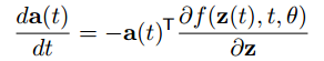（1）
该等式在1962年由 Pontryagin et al. 的论文《The mathematical theory of optimal processes》给出过证明，不过，本文作者也给出了相应的更简洁的证明过程：
  对于连续的隐层状态，可以将在时间上变化后的 ε \varepsilon ε 记作：
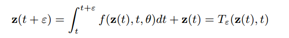（2）
上述公式说明，下一个状态 z z z 是关于上一个状态的函数（这里将参数 θ \theta θ 看作常量，具体的积分值由 f f f 决定）。 因此，相应的链式法则可以记作：
（3）
由此，可以证明（1）式：

通过上述证明过程（引入 T ε ( z ( t ) ) T_{\varepsilon}(z(t)) Tε​(z(t)) ,以说明 z ( t + ε ) z(t+\varepsilon) z(t+ε) 是 z ( t ) z(t) z(t)的函数），第二步用到等式（3），另外对等式（2）进行泰勒展开（ T ε T_{\varepsilon} Tε​ 中的 t t t 被隐含了），注意展开过程中的无穷小参数同样取 ε \varepsilon ε，然后就可以得到等式（1）。

  We specify the constraint on the last time point, which is simply the gradient of the loss wrt the last time point, and can obtain the gradients with respect to the hidden state at any time, including the initial value.

  这里就可以看出 ODE 沿时间的反向过程和 NN 中反向传播（BP）的相似性了。也就是通过 ODE 系统，前向和后向都是可以计算的。这里假设（限制）最后时刻（ T N T_N TN​）的隐层状态是已知的（可以直接通过 loss 的梯度获取），就可以求解任意时刻的隐层状态了（包括初始时刻）：

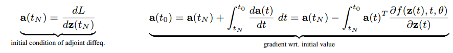
  由此，整个 ODE 的反向过程的理论部分证明完成。

  这里引入了一个伴随状态（Adjoint State），它和前向状态相反，通过另一个 ODE 来求解。 关键是它们是怎样建立联系的？见下图：

  The adjoint sensitivity method solves an augmented ODE backwards in time. The augmented system contains both the original state and the sensitivity of the loss with respect to the state.
  伴随敏感度方法使用一个增强的在时间上反向的 ODE。该增强系统同时包括 原来的状态 a ( t ) a(t) a(t) 和损失对该状态的敏感度 ∂ L a ( t ) ∂ z ( t N ) \frac{\partial La(t)}{\partial {z(t_N)}} ∂z(tN​)∂La(t)​。具体它俩是怎么计算的？
  答案是：由损失敏感度 ∂ L a ( t ) ∂ z ( t N ) \frac{\partial La(t)}{\partial {z(t_N)}} ∂z(tN​)∂La(t)​ 调节伴随（adjoint）状态 a ( t ) a(t) a(t)， 然后再有伴随状态 a ( t ) a(t) a(t) 得到损失敏感度 ∂ L a ( t ) ∂ z ( t N ) \frac{\partial La(t)}{\partial {z(t_N)}} ∂z(tN​)∂La(t)​ 。这是 ODE 反向的链式过程。至此，整个反向传播的过程就被模拟了！

  Computing the gradients with respect to the parameters θ requires evaluating a third integral, which depends on both z(t) and a(t):
  计算关于 θ \theta θ 的梯度，还要计算相关变量 z(t) and a(t) 的积分：
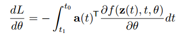（4）

  通过等式（1）和（4）就可以计算出梯度了， a ( t ) T ∂ f ∂ z {a(t)}^T \frac{\partial f}{\partial z} a(t)T∂z∂f​ 和 a ( t ) T ∂ f ∂ θ {a(t)}^T \frac{\partial f}{\partial \theta} a(t)T∂θ∂f​ 的vector-Jacobian products 都可以通过 ODE solver 快速求解。 所有的积分解： z , a , ∂ L ∂ θ z, a, \frac{\partial L}{\partial \theta} z,a,∂θ∂L​ 都可以通过一个 ODE solver 来求解，可以将它们组合成一个向量解 (增强的状态，augmented state)。具体步骤见算法 1：

该算法基本上是上述过程的综合。首先定义初始状态 s 0 s_0 s0​，然后定义 增强状态，aug_dynamics，该状态包括 f ( z ( t ) , t , θ ) f(z(t),t,\theta) f(z(t),t,θ)， a ( t ) T ∂ f ∂ z {a(t)}^T \frac{\partial f}{\partial z} a(t)T∂z∂f​ 和 a ( t ) T ∂ f ∂ θ {a(t)}^T \frac{\partial f}{\partial \theta} a(t)T∂θ∂f​ 的vector-Jacobian products（通过自动微分工具得到）。然后通过 ODE solver 求解前一时刻的隐层状态，敏感状态，和梯度。注意，这些都是合并起来的向量形式（算子形式的张量？）。最后，返回敏感状态(用以下一时刻计算敏感状态)和梯度（用以更新参数 θ \theta θ）。

---

Replacing residual networks with ODEs

将ResNets 换成 ODEs

  Software: To solve ODE initial value problems numerically, we use the implicit Adams method implemented in LSODE and VODE and interfaced through the scipy.integrate package. Being an implicit method, it has better guarantees than explicit methods such as Runge-Kutta but requires solving a nonlinear optimization problem at every step.This setup makes direct backpropagation through the integrator difficult.

  软件实现： 为了求解 ODE 的数值解， 作者使用 Adams （一种梯度优化方法）方法实现了 LSODE 和 VODE 的scipy.integrate 接口。 作为一种隐式方法，它比显式方法有较好的保证，如 Runge-Kutta 需要在每一步求解非线性优化问题。这种设置使得直接使用积分器求解反向传播是困难的。作者使用 Python 的自动微分方法实现了伴随敏感方法，并使用 Tensorflow 在GPU上实现了 隐层状态的动态和求导（从Fortran ODE Solver 调用，从 Python autograd 中调用）。

  Model Architectures: We experiment with a small residual network which downsamples the input twice then applies 6 standard residual blocks He et al. (2016b), which are replaced by an ODESolve module in the ODE-Net variant. We also test a network with the same architecture but where gradients are backpropagated directly through a Runge-Kutta integrator, referred to as RK-Net.

  论文中用两个降采样和6个残差块的小型 ResNet 进行了实验，将残差块替换为ODESolve 模块就变成了 ODE-Net 变体。作者还使用相同的架构测试了使用 Runge-Kutta 积分器来反向传播梯度的 RK-Net。

  代码实现

首先看整体网络结构：

feature_layers = [ODEBlock(ODEfunc(64))] if is_odenet else [ResBlock(64, 64) for _ in range(6)]

其中,ODEfunc 定义为：

class ODEfunc(nn.Module):

    def __init__(self, dim):
        super(ODEfunc, self).__init__()
        self.norm1 = norm(dim)
        self.relu = nn.ReLU(inplace=True)
        self.conv1 = ConcatConv2d(dim, dim, 3, 1, 1)
        self.norm2 = norm(dim)
        self.conv2 = ConcatConv2d(dim, dim, 3, 1, 1)
        self.norm3 = norm(dim)
        self.nfe = 0 # number of forward ?

    def forward(self, t, x):
        self.nfe += 1
        out = self.norm1(x)
        out = self.relu(out)
        out = self.conv1(t, out)
        out = self.norm2(out)
        out = self.relu(out)
        out = self.conv2(t, out)
        out = self.norm3(out)
        return out

  与 Residual Block 不同的是多加了一次 Batch Normalization，ODEfunc 中的卷积 ConcatConv2d 实现为：

class ConcatConv2d(nn.Module):

    def __init__(self, dim_in, dim_out, ksize=3, stride=1, padding=0, dilation=1, groups=1, bias=True, transpose=False):
        super(ConcatConv2d, self).__init__()
        module = nn.ConvTranspose2d if transpose else nn.Conv2d
        self._layer = module(
            dim_in + 1, dim_out, kernel_size=ksize, stride=stride, padding=padding, dilation=dilation, groups=groups,
            bias=bias
        )

    def forward(self, t, x):
        tt = torch.ones_like(x[:, :1, :, :]) * t   # extract the first channel and multiply the time t.
        ttx = torch.cat([tt, x], 1)
        return self._layer(ttx)

  可以看到 ConcatConv2d 和原来的 卷积方式 基本相同，只是在 前向过程中，添加了变量（variable） t t t , 其中，torch.ones_like 返回一个填充了标量值1的张量，其大小与之相同 input ，乘以 t t t 表示在 t t t 时刻。然后，将 t t t 与 x x x 合并（concatenation）起来，然后作为卷积的输入。这里有个问题，为什么变量 t t t 的 size 是 feature size，难道是对每个feature position 做连续化？//TODO （这里 grad 的形状和feature size 的形状相同）。

  接下来就是 ODEBlock的定义：

class ODEBlock(nn.Module):

    def __init__(self, odefunc):
        super(ODEBlock, self).__init__()
        self.odefunc = odefunc
        self.integration_time = torch.tensor([0, 1]).float()

    def forward(self, x):
        self.integration_time = self.integration_time.type_as(x)
        out = odeint(self.odefunc, x, self.integration_time, rtol=args.tol, atol=args.tol) # ODE forward
        return out[1]

  ODEBlock 中定义了 积分时间（integration time） t ∈ [ 0 , 1 ] t \in [0,1] t∈[0,1] ，然后在前向过程中传入 odeint 中，关键点是 odeint, 按上述算法中。这里 rtol 和 atol 是 容忍度（tolerance），即模型的精度设定。out[1] 是梯度（gradient） ∂ L ∂ θ \frac{\partial L}{\partial \theta} ∂θ∂L​。这样我们求得了梯度。其中，odeint 的实现为：

def odeint(func, y0, t, rtol=1e-7, atol=1e-9, method=None, options=None):
      tensor_input, func, y0, t = _check_inputs(func, y0, t)

    if options is None:
        options = {}
    elif method is None:
        raise ValueError('cannot supply `options` without specifying `method`')

    if method is None:
        method = 'dopri5'

    solver = SOLVERS[method](func, y0, rtol=rtol, atol=atol, **options)
    solution = solver.integrate(t)

    if tensor_input:
        solution = solution[0]
    return solution

The goal of an ODE solver is to find a continuous trajectory satisfying the ODE that passes through the initial condition. Solves the initial value problem （IVP） for a non-stiff system of first order ODEs: ∂ y ∂ t = f ( t , y ) \frac{\partial y}{\partial t}=f(t,y) ∂t∂y​=f(t,y) s.t. y ( t 0 ) = y 0 y(t_0)=y_0 y(t0​)=y0​ where y is a Tensor of any shape.

odeint 解的是非复杂（non-stiff）系统的一阶 ODE 的初值问题 (IVP)，其中，y是任意形状的张量。以下是其中参数的解释：

"""
	Args:
        func: Function that maps a Tensor holding the state `y` and a scalar Tensor
            `t` into a Tensor of state derivatives with respect to time.
    func：把一个含有状态张量 y 和常张量 t 映射到 一个关于时间可导的张量上。
        y0: N-D Tensor giving starting value of `y` at time point `t[0]`. May
            have any floating point or complex dtype.
    y0: NxD维度的张量，是 y 在 t[0] 的初始点，可以是任意复杂的类型。
        t: 1-D Tensor holding a sequence of time points for which to solve for
            `y`. The initial time point should be the first element of this sequence,
            and each time must be larger than the previous time. May have any floating
            point dtype. Converted to a Tensor with float64 dtype.
    t: 1xD的张量，表示一系列用于求解 y 的时间点。
        rtol: optional float64 Tensor specifying an upper bound on relative error,
            per element of `y`.
    rtol: 相对错误容忍度，以限制张量 y 中每个元素的上限值。（可调节）
        atol: optional float64 Tensor specifying an upper bound on absolute error,
            per element of `y`.
    atol: 绝对错误容忍度，以限制张量 y 中每个元素的上限值。（可调节）
        method: optional string indicating the integration method to use.
        method: 可选的string型 以决定那种 积分方法 被使用。
        options: optional dict of configuring options for the indicated integration
            method. Can only be provided if a `method` is explicitly set.
    options: 可选的字典类型，用于配置积分方法。
        name: Optional name for this operation.
	name:  为该操作指定名称。
    Returns:
        y: Tensor, where the first dimension corresponds to different
            time points. Contains the solved value of y for each desired time point in
            `t`, with the initial value `y0` being the first element along the first
            dimension.
    Returns: 返回第一个维度对应不同的时间点的 y 张量。
             包含 y 在每个时间点 t 上被期望的解。（所有时间点的解都被求得了），
             初始值 y0 是第一维度的第一个元素。
"""

  看一下 SOLOVE中的积分方法：

SOLVERS = {
    'explicit_adams': AdamsBashforth,
    'fixed_adams': AdamsBashforthMoulton,
    'adams': VariableCoefficientAdamsBashforth,
    'tsit5': Tsit5Solver,
    'dopri5': Dopri5Solver,
    'euler': Euler,
    'midpoint': Midpoint,
    'rk4': RK4,
}

  这里牵涉到微分方程的数值解法。这里 AdamsBashforth、AdamsBashforthMoulton、Euler、Midpoint、RK4 (Fourth-order Runge-Kutta with 3/8 rule) 属于 FixedGridODESolver (固定网格 ODE 求解器)，其中，前两个 Adams 类型的求解器 是作者自己实现的 Adam梯度下降方法来求解的 FixedGridODESolver。而VariableCoefficientAdamsBashforth、Tsit5Solver （）、Dopri5Solver （Runge-Kutta 4(5)）属于 AdaptiveStepsizeODESolver（自定义步长的 ODE 求解器）。论文中把 ODE solver 当作一个黑盒子（black box），我们知道它可以求解我们所需要的微分方程。这里只看最简单的 Euler 求解器：

class Euler(FixedGridODESolver):

    def step_func(self, func, t, dt, y):
        return tuple(dt * f_ for f_ in func(t, y))

  它只是实现了父类 FixedGridODESolver 中的 step_func，父类 FixedGridODESolver 的实现为：

class FixedGridODESolver(object):
	def __init__(self, func, y0, step_size=None, grid_constructor=None, **unused_kwargs):
		...
		... # here, I omit some initialize progress in origin code
		# and omit some grid constructor progress.
		 
	@abc.abstractmethod
    def step_func(self, func, t, dt, y):
        pass

    def integrate(self, t):
        _assert_increasing(t) # t is increase sequence
        t = t.type_as(self.y0[0])
        time_grid = self.grid_constructor(self.func, self.y0, t) # grad
        assert time_grid[0] == t[0] and time_grid[-1] == t[-1]
        time_grid = time_grid.to(self.y0[0])

        solution = [self.y0] # target solution list

        j = 1
        y0 = self.y0
        for t0, t1 in zip(time_grid[:-1], time_grid[1:]):
            dy = self.step_func(self.func, t0, t1 - t0, y0) # use step function
            y1 = tuple(y0_ + dy_ for y0_, dy_ in zip(y0, dy)) # y1=y0+dy
            y0 = y1 # why to this?
			# linear interpolate the time sequence.
            while j < len(t) and t1 >= t[j]:
                solution.append(self._linear_interp(t0, t1, y0, y1, t[j]))
                j += 1

        return tuple(map(torch.stack, tuple(zip(*solution))))
        
    def _linear_interp(self, t0, t1, y0, y1, t):
        if t == t0:
            return y0
        if t == t1:
            return y1
        t0, t1, t = t0.to(y0[0]), t1.to(y0[0]), t.to(y0[0])
        slope = tuple((y1_ - y0_) / (t1 - t0) for y0_, y1_, in zip(y0, y1))
        return tuple(y0_ + slope_ * (t - t0) for y0_, slope_ in zip(y0, slope))

  这里的积分 应该是对 差分 的积分，即根据初始值 y 0 y_0 y0​ 和时间序列 t t t 来求 y t y_t yt​。 首先构建 time grad，然后使用step_func，根据 func (NN 中的 f f f) 和 time grad 中的 t 以及 y 0 y_0 y0​ 来计算 d y dy dy, 接着，根据 y 1 = y 0 + d y y_1=y_0+dy y1​=y0​+dy 求得 y 1 y_1 y1​, 这里有一行 y 0 = y 1 y_0=y_1 y0​=y1​, 为什么把y1赋值给 y 0 y_0 y0​ ? 然后再根据 y 0 y_0 y0​, y 1 y_1 y1​ 求插值 ？这样元素不就等于零了？ //todo

  到这里，整个 ODE-Net的方法和实现都走一遍了，但我们好像只看到了前向过程？没有反向过程？这是因为 反向过程被 Pytorch 在内部自动实现了 （autograd backpropagate），并没有使用作者提出的 adjoint sensitivity method。作者指出使用 adjoint 方法可将 内存复杂度 降为 O ( 1 ) O(1) O(1)。

  Backpropagation through odeint goes through the internals of the solver, but this is not supported for all solvers. Instead, we encourage the use of the adjoint method, which will allow solving with as many steps as necessary due to O(1) memory usage.

  odeint_adjoint simply wraps around odeint, but will use only O(1) memory in exchange for solving an adjoint ODE in the backward call. The biggest gotcha is that func must be a nn.Module when using the adjoint method. This is used to collect parameters of the differential equation.

odeint_adjoint 简单第封装了 odeint，并实现了反向过程。但其最大的缺憾（硬伤）是func f f f 的取值必须是 nn.Module 的方法，这是为了收集微分方程的参数。( Why must be collect parameters of the differential equation? The answer is use to backward of adjoint odeint.）看一下adjoint odeint 的实现过程：

def odeint_adjoint(func, y0, t, rtol=1e-6, atol=1e-12, method=None, options=None):

    # We need this in order to access the variables inside this module,
    # since we have no other way of getting variables along the execution path.
    if not isinstance(func, nn.Module):
        raise ValueError('func is required to be an instance of nn.Module.')

    tensor_input = False
    if torch.is_tensor(y0):

        class TupleFunc(nn.Module):

            def __init__(self, base_func):
                super(TupleFunc, self).__init__()
                self.base_func = base_func

            def forward(self, t, y):
                return (self.base_func(t, y[0]),)

        tensor_input = True
        y0 = (y0,)
        func = TupleFunc(func)

    flat_params = _flatten(func.parameters())
    ys = OdeintAdjointMethod.apply(*y0, func, t, flat_params, rtol, atol, method, options)

    if tensor_input:
        ys = ys[0]
    return ys

  首先说明了odeint_adjoint 的变量是有序的，然后通过内部类封装了一下 func，这里明确的限制了 func 是 nn.Module，这样 ODE-Net 的前向过程就实现了。接下来，通过 OdeintAdjointMethod 具体执行 ODE 的前向和反向过程：

class OdeintAdjointMethod(torch.autograd.Function):

    @staticmethod
    def forward(ctx, *args):
        assert len(args) >= 8, 'Internal error: all arguments required.'
        y0, func, t, flat_params, rtol, atol, method, options = \
            args[:-7], args[-7], args[-6], args[-5], args[-4], args[-3], args[-2], args[-1]

        ctx.func, ctx.rtol, ctx.atol, ctx.method, ctx.options = func, rtol, atol, method, options

        with torch.no_grad():
            ans = odeint(func, y0, t, rtol=rtol, atol=atol, method=method, options=options)
        ctx.save_for_backward(t, flat_params, *ans)
        return ans

  前向过程很简单，通过继承 torch.autograd.Function，将一些参数赋值给 ctx（没有通过 self 实现，因为ctx只在forward过程中存在。通过 self 会不会更直观），并保存了 t t t，func 的参数 和 odeint 的前向结果，以便在反向过程中使用。再看其反向过程：

    @staticmethod
    def backward(ctx, *grad_output):

        t, flat_params, *ans = ctx.saved_tensors
        ans = tuple(ans)
        func, rtol, atol, method, options = ctx.func, ctx.rtol, ctx.atol, ctx.method, ctx.options
        n_tensors = len(ans)
        f_params = tuple(func.parameters())

        # TODO: use a nn.Module and call odeint_adjoint to implement higher order derivatives.
        def augmented_dynamics(t, y_aug):
            # Dynamics of the original system augmented with
            # the adjoint wrt y, and an integrator wrt t and args.
            y, adj_y = y_aug[:n_tensors], y_aug[n_tensors:2 * n_tensors]  # Ignore adj_time and adj_params.

            with torch.set_grad_enabled(True):
                t = t.to(y[0].device).detach().requires_grad_(True)
                y = tuple(y_.detach().requires_grad_(True) for y_ in y)
                func_eval = func(t, y)
                vjp_t, *vjp_y_and_params = torch.autograd.grad(
                    func_eval, (t,) + y + f_params,
                    tuple(-adj_y_ for adj_y_ in adj_y), allow_unused=True, retain_graph=True
                )
            vjp_y = vjp_y_and_params[:n_tensors]
            vjp_params = vjp_y_and_params[n_tensors:]

            # autograd.grad returns None if no gradient, set to zero.
            vjp_t = torch.zeros_like(t) if vjp_t is None else vjp_t
            vjp_y = tuple(torch.zeros_like(y_) if vjp_y_ is None else vjp_y_ for vjp_y_, y_ in zip(vjp_y, y))
            vjp_params = _flatten_convert_none_to_zeros(vjp_params, f_params)

            if len(f_params) == 0:
                vjp_params = torch.tensor(0.).to(vjp_y[0])
            return (*func_eval, *vjp_y, vjp_t, vjp_params)

        T = ans[0].shape[0]
        with torch.no_grad():
            adj_y = tuple(grad_output_[-1] for grad_output_ in grad_output)
            adj_params = torch.zeros_like(flat_params)
            adj_time = torch.tensor(0.).to(t)
            time_vjps = []
            for i in range(T - 1, 0, -1):

                ans_i = tuple(ans_[i] for ans_ in ans)
                grad_output_i = tuple(grad_output_[i] for grad_output_ in grad_output)
                func_i = func(t[i], ans_i)

                # Compute the effect of moving the current time measurement point.
                dLd_cur_t = sum(
                    torch.dot(func_i_.reshape(-1), grad_output_i_.reshape(-1)).reshape(1)
                    for func_i_, grad_output_i_ in zip(func_i, grad_output_i)
                )
                adj_time = adj_time - dLd_cur_t
                time_vjps.append(dLd_cur_t)

                # Run the augmented system backwards in time.
                if adj_params.numel() == 0:
                    adj_params = torch.tensor(0.).to(adj_y[0])
                aug_y0 = (*ans_i, *adj_y, adj_time, adj_params)
                aug_ans = odeint(
                    augmented_dynamics, aug_y0,
                    torch.tensor([t[i], t[i - 1]]), rtol=rtol, atol=atol, method=method, options=options
                )

                # Unpack aug_ans.
                adj_y = aug_ans[n_tensors:2 * n_tensors]
                adj_time = aug_ans[2 * n_tensors]
                adj_params = aug_ans[2 * n_tensors + 1]

                adj_y = tuple(adj_y_[1] if len(adj_y_) > 0 else adj_y_ for adj_y_ in adj_y)
                if len(adj_time) > 0: adj_time = adj_time[1]
                if len(adj_params) > 0: adj_params = adj_params[1]

                adj_y = tuple(adj_y_ + grad_output_[i - 1] for adj_y_, grad_output_ in zip(adj_y, grad_output))

                del aug_y0, aug_ans

            time_vjps.append(adj_time)
            time_vjps = torch.cat(time_vjps[::-1])

            return (*adj_y, None, time_vjps, adj_params, None, None, None, None, None)

  其中，torch.autograd.grad(outputs, inputs, grad_outputs=None, … ) 是用来计算输出对输入的梯度（Computes and returns the sum of gradients of outputs w.r.t. the inputs.）。这里需要用到 自动微分 中的知识。