3.4 数据变换
请参考《数据准备和特征工程》中的相关章节,调试如下代码。

基础知识
import pandas as pd

data = pd.read_csv("/home/aistudio/data/data20514/freefall.csv", index_col=0)
data.describe()
|
time |
location |
| count |
100.000000 |
1.000000e+02 |
| mean |
250.000000 |
4.103956e+05 |
| std |
146.522832 |
3.709840e+05 |
| min |
0.000000 |
0.000000e+00 |
| 25% |
124.997500 |
7.658593e+04 |
| 50% |
250.000000 |
3.062812e+05 |
| 75% |
375.002500 |
6.890859e+05 |
| max |
500.000000 |
1.225000e+06 |
# !mkdir /home/aistudio/external-libraries
# !pip install -i https://pypi.tuna.tsinghua.edu.cn/simple seaborn -t /home/aistudio/external-libraries
import sys
sys.path.append('/home/aistudio/external-libraries')
%matplotlib inline
import seaborn as sns

# scatterplot绘制散点图
ax = sns.scatterplot(x='time', y='location', data=data)

import numpy as np
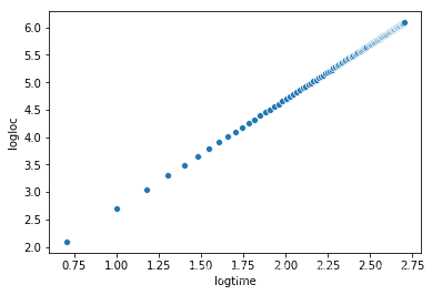
data.drop([0], inplace=True) # 去掉0,不计算log0
data['logtime'] = np.log10(data['time']) # 求对数
data['logloc'] = np.log10(data['location'])
data.head()
|
time |
location |
logtime |
logloc |
| 1 |
5.05 |
124.99 |
0.703291 |
2.096875 |
| 2 |
10.10 |
499.95 |
1.004321 |
2.698927 |
| 3 |
15.15 |
1124.89 |
1.180413 |
3.051110 |
| 4 |
20.20 |
1999.80 |
1.305351 |
3.300987 |
| 5 |
25.25 |
3124.68 |
1.402261 |
3.494806 |
ax2 = sns.scatterplot(x='logtime', y='logloc', data=data)
from sklearn.linear_model import LinearRegression

reg = LinearRegression()
reg.fit(data[['logtime']], data[['logloc']])

# 返回直线的斜率和截距
(reg.coef_, reg.intercept_)
(array([[1.99996182]]), array([0.69028797]))
import numpy as np

X = np.arange(6).reshape(3, 2)
X
array([[0, 1],
       [2, 3],
       [4, 5]])
from sklearn.preprocessing import PolynomialFeatures

# 多项式变换,2代表创建一个最高项为2的多项式:1 + x1 + x2 + x1*x1 + x1*x2 + x2*x2
poly = PolynomialFeatures(2)

# 将x1和x2依次代入行向量中,从而得到一个更大的特征矩阵
poly.fit_transform(X)
array([[ 1.,  0.,  1.,  0.,  0.,  1.],
       [ 1.,  2.,  3.,  4.,  6.,  9.],
       [ 1.,  4.,  5., 16., 20., 25.]])
项目案例
dc_data = pd.read_csv('/home/aistudio/data/data20514/sample_data.csv')
dc_data.head()
|
MONTH |
AIR_TIME |
| 0 |
1 |
28 |
| 1 |
1 |
29 |
| 2 |
1 |
29 |
| 3 |
1 |
29 |
| 4 |
1 |
29 |
%matplotlib inline
import matplotlib.pyplot as plt
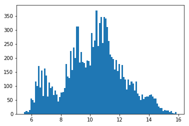
# 绘制特征“AIR_TIME”的直方图,看是否符合正态分布
h = plt.hist(dc_data['AIR_TIME'], bins=100)

from scipy import stats
# 将特征AIR_TIME转换为二维矩阵,便于输入
transform = dc_data[['AIR_TIME']]
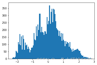
# 通过boxcox变换,将其变为正态分布
dft = stats.boxcox(transform)[0]
# 检查是否符合正态分布
hbc = plt.hist(dft, bins=100)
from sklearn.preprocessing import power_transform

# power_transform:广义幂变换,它包含了:box-cox变换和yeo-johnson变换
dft2 = power_transform(dc_data[['AIR_TIME']], method='box-cox')

hbcs = plt.hist(dft2, bins=100)
动手练习
%matplotlib inline
import pandas as pd
import matplotlib.pyplot as plt
from sklearn.linear_model import Ridge
from sklearn.preprocessing import PolynomialFeatures
from sklearn.pipeline import make_pipeline
df = pd.read_csv("/home/aistudio/data/data20514/xsin.csv")
colors = ['teal', 'yellowgreen', 'gold']
# 绘制散点图
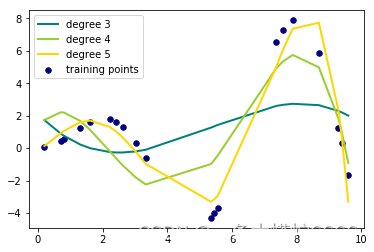
plt.scatter(df['x'], df['y'], color='navy', s=30, marker='o', label="training points")
for count, degree in enumerate([3, 4, 5]):
# PolynomialFeatures(),多项式变换
# Ridge(),线性最小二乘L2正则化。该模型求解了线性最小二乘函数和L2正则化的回归模型。也称为岭回归或者Tikhonov 正则化。
# make_pipeline可以将许多算法模型串联起来,比如将特征提取、归一化、分类组织在一起形成一个典型的机器学习问题工作流。
model = make_pipeline(PolynomialFeatures(degree), Ridge()) # 获得岭回归后的模型
model.fit(df[['x']], df[['y']]) # 用真实数据来训练模型
y_pre = model.predict(df[['x']]) # 通过训练好的模型来预测y值
# 绘制预测图表,不难发现degree=4是与原数据集拟合的最好的
plt.plot(df['x'], y_pre, color=colors[count], linewidth=2,
label="degree %d" % degree)
# 绘制左上角的图例
plt.legend()