【优化求解】基于粒子群算法集合生物地理算法CPSOBBO求解MLP问题matlab代码

1 简介

Biogeography-Based Optimizer (BBO) is employed as a trainer for Multi-Layer Perceptron (MLP). The current source codes are the demonstration of the BBO-MLP trainer for solving the Iris classification problem. There are also other trainers in this submission: Particle Swarm Optimization (PSO), Ant Colony Optimization (ACO), Genetic Algorithm (GA), Evolutionary Strategy (ES), and Probability-Based Incremental Learning (PBIL). The classification accuracy of BBO-MLP is calculated at the end of main.m file and compared to those of PSO, ACO, ES, GA, and PBIL. The convergence curve and classification accuracy of each algorithm are drawn at the end.

2 部分代码

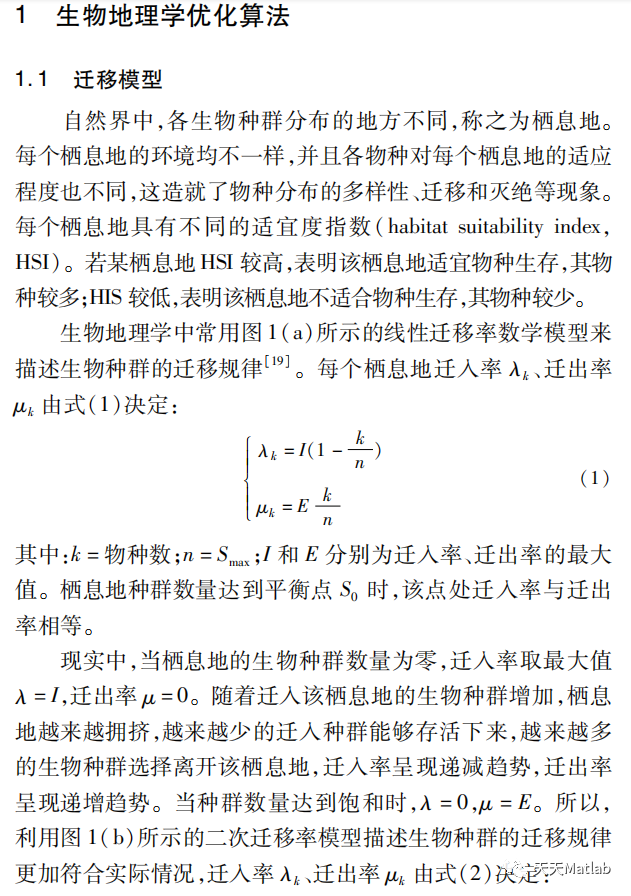
%%%%% Multi-layer Perceptron (MLP) Training using CPSOGSA %%%%%

clear all
close all
clc
Q=1;            % ACO Parameter
tau0=10;        % Initial Phromone             (ACO)
alpha=0.3;      % Phromone Exponential Weight (ACO)
rho=0.1;        % Evaporation Rate             (ACO)
beta_min=0.2;   % Lower Bound of Scaling Factor (DE)
beta_max=0.8;   % Upper Bound of Scaling Factor (DE)
pCR=0.2;        % Crossover Probability         (DE)
Runno=10;

SearchAgents_no=20; % Number of search agents

% classification datasets

Function_name='F2'; %MLP_Baloon dataset
% Load details of the selected data set
[lb,ub,dim,fobj]=Get_Functions_details(Function_name);
ElitistCheck=1;
min_flag=1;
Rpower=1;
Max_iteration=500; % Maximum numbef of iterations
%

load baloon.txt
x=sortrows(baloon,2);
%I2=x(1:150,1:4);
I2(:,1)=x(1:20,1);
I2(:,2)=x(1:20,2);
I2(:,3)=x(1:20,3);
I2(:,4)=x(1:20,4);
T=x(1:20,5);


Hno=9;
dim = 6*9+1;

for i=1:1:Runno
  [Fbest,Lbest,BestChart]=GSA(SearchAgents_no,Max_iteration,ElitistCheck,min_flag,Rpower,lb,ub,dim,fobj);
   BestSolutions1(i) = Fbest;
  [gBestScore,gBest,GlobalBestCost]= CPSOGSA(SearchAgents_no,Max_iteration,lb,ub,dim,fobj);
   BestSolutions4(i) = gBestScore;
  [BestSolACO,BestAnt,BestCostACO] = ACO(SearchAgents_no, Max_iteration,Q,tau0,alpha,rho,lb,ub,dim,fobj);
   BestSolutions5(i) = BestSolACO.Cost;
  [BestCost,Best_Hab,BestSol] = bbo( SearchAgents_no, Max_iteration,lb,ub,dim,fobj);
   BestSolutions6(i) = BestSol.Cost;
  [BestSolDE,DBestSol,BestCostDE] = DE(SearchAgents_no, Max_iteration,beta_min,beta_max,pCR,lb,ub,dim,fobj);
   BestSolutions7(i) = BestSolDE.Cost ;
   Rrate=0;
   
   W=Lbest(1:45);
   B=Lbest(46:55);
   W=gBest(1:45);
   B=gBest(46:55);
   W=BestAnt(1:45);
   B=BestAnt(46:55);
   W=Best_Hab(1:45);
   B=Best_Hab(46:55);
   W=DBestSol(1:45);
   B=DBestSol(46:55);
   
   for pp=1:20
       actualvalue=my_simulate(4,9,1,W,B,I2(pp,:));
       if(T(pp)==1)
           if (actualvalue>=0.95)
               Rrate=Rrate+1;
           end
       end
       if(T(pp)==0)
           if (actualvalue(1)<0.05)
               Rrate=Rrate+1;
           end
       end
       
   end
end

% % %
figure
semilogy(1:Max_iteration,BestChart,'DisplayName','GSA','Color','g','Marker','o','LineStyle','-','LineWidth',2,...
   'MarkerEdgeColor','g','MarkerFaceColor',[.49 1 .63],'MarkerSize',5);
hold on

semilogy(1:Max_iteration,GlobalBestCost,'DisplayName','CPSOGSA', 'Color', 'r','Marker','diamond','LineStyle','-','LineWidth',2,...
   'MarkerEdgeColor','r','MarkerFaceColor',[.49 1 .63],'MarkerSize',5);
% semilogy(1:Max_iteration,BestCostACO,'DisplayName','ACO','Color','c','Marker','square','LineStyle','-','LineWidth',2,...
%     'MarkerEdgeColor','c','MarkerFaceColor',[.49 1 .63],'MarkerSize',5);
% semilogy(1:Max_iteration,BestCost,'DisplayName','BBO','Color','b','Marker','*','LineStyle','-','LineWidth',2,...
%     'MarkerEdgeColor','b','MarkerFaceColor',[.49 1 .63],'MarkerSize',5);
% semilogy(1:Max_iteration,BestCostDE,'DisplayName','DE','Color','y','Marker','+','LineStyle','-','LineWidth',2,...
%     'MarkerEdgeColor','y','MarkerFaceColor',[.49 1 .63],'MarkerSize',5);

title ('\fontsize{12}\bf XOR Dataset');

% title ('\fontsize{12}\bf Baloon Dataset');
% title ('\fontsize{12}\bf Iris Dataset');
% title ('\fontsize{12}\bf Cancer Dataset');
% title ('\fontsize{12}\bf Heart Dataset');
% title ('\fontsize{12}\bf Sigmoid Dataset');
% title ('\fontsize{12}\bf Cosine Dataset');
% title ('\fontsize{12}\bf Sine Dataset');

xlabel('\fontsize{12}\bf Iteration');
ylabel('\fontsize{12}\bf log(MSE)');
legend('\fontsize{10}\bf GSA','\fontsize{10}\bf CPSOGSA')
% legend('\fontsize{10}\bf GSA','\fontsize{10}\bf CPSOGSA','\fontsize{10}\bf ACO','\fontsize{10}\bf BBO','\fontsize{10}\bf DE',1);

axis tight
box on

img =gcf;  %获取当前画图的句柄
print(img, '-dpng', '-r600', './img.png')         %即可得到对应格式和期望dpi的图像

3 仿真结果

4 参考文献

S. Mirjalili, S. M. Mirjalili, A. Lewis, Let A Biogeography-Based Optimizer Train Your Multi-Layer Perceptron, Information Sciences, In press, 2014