Tensorflow学习笔记（一）

Tensorflow

Tensorflow官方教程

由于Google Colab在国内无法使用，推荐deepnote代替

基本分类：对服装图像进行分类

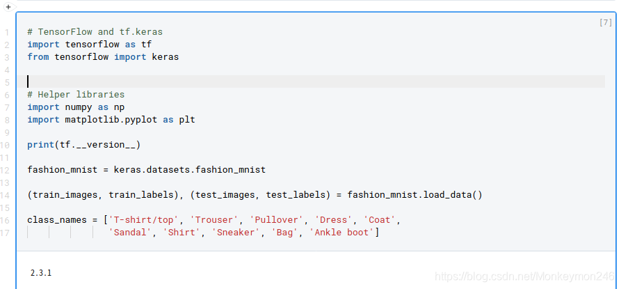
# TensorFlow and tf.keras
import tensorflow as tf
from tensorflow import keras

# Helper libraries
import numpy as np
import matplotlib.pyplot as plt

print(tf.__version__)

fashion_mnist = keras.datasets.fashion_mnist

(train_images, train_labels), (test_images, test_labels) = fashion_mnist.load_data()

class_names = ['T-shirt/top', 'Trouser', 'Pullover', 'Dress', 'Coat',
               'Sandal', 'Shirt', 'Sneaker', 'Bag', 'Ankle boot']

plt.figure()
plt.imshow(train_images[0])
plt.colorbar()
plt.grid(False)
plt.show()

train_images = train_images / 255.0

test_images = test_images / 255.0

plt.figure(figsize=(10,10))
for i in range(25):
    plt.subplot(5,5,i+1)
    plt.xticks([])
    plt.yticks([])
    plt.grid(False)
    plt.imshow(train_images[i], cmap=plt.cm.binary)
    plt.xlabel(class_names[train_labels[i]])
plt.show()

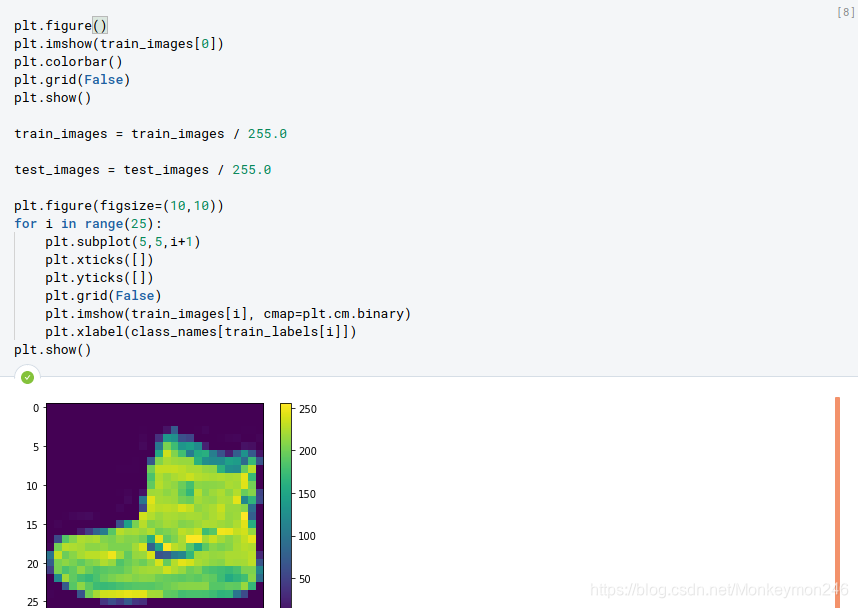
画图前：先使用 plt.figure() 来新创一个图片或者激活已经有的图片，而plt.colorbar()可以在图上加上那个深浅棒，plt.show()画出所有打开的图片

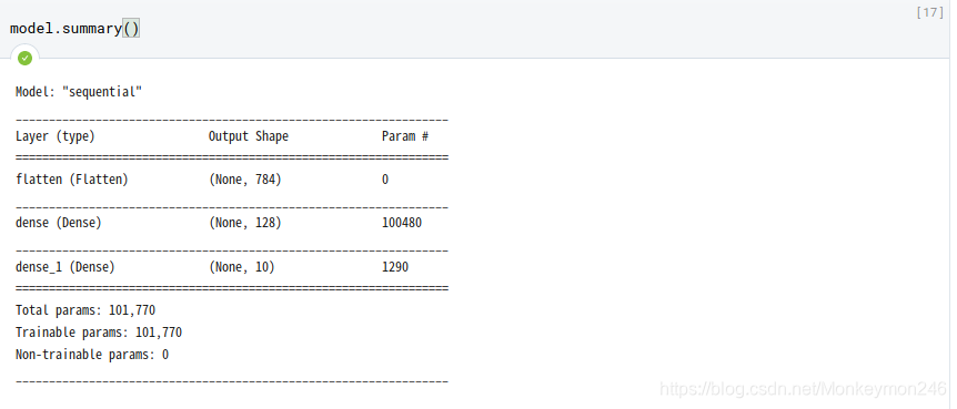
model = keras.Sequential([
    keras.layers.Flatten(input_shape=(28, 28)),
    keras.layers.Dense(128, activation='relu'),
    keras.layers.Dense(10)
])
model.compile(optimizer='adam',
              loss=tf.keras.losses.SparseCategoricalCrossentropy(from_logits=True),
              metrics=['accuracy'])
              
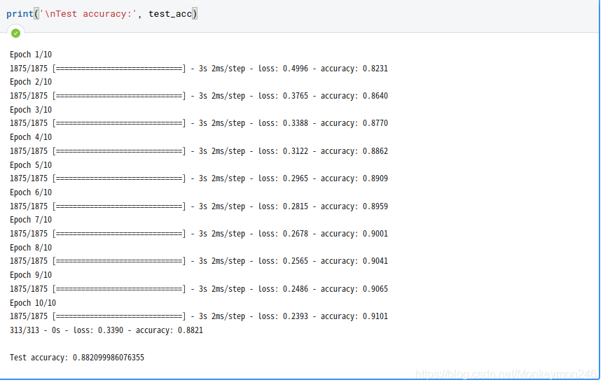
model.fit(train_images, train_labels, epochs=10)
test_loss, test_acc = model.evaluate(test_images,  test_labels, verbose=2)

print('\nTest accuracy:', test_acc)

probability_model = tf.keras.Sequential([model, 
                                         tf.keras.layers.Softmax()])
predictions = probability_model.predict(test_images)
print(predictions)

这里有一个很有意思的事情，probability_model 是补充在model后的，按照正常的模型构建，理所当然以为应该在compile和fit前面，那是因为这层没有用到参数

同理，flatten那层也没有用到参数

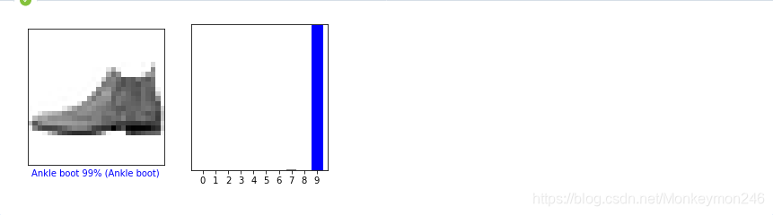
def plot_image(i, predictions_array, true_label, img):
  predictions_array, true_label, img = predictions_array, true_label[i], img[i]
  plt.grid(False)
  plt.xticks([])
  plt.yticks([])

  plt.imshow(img, cmap=plt.cm.binary)

  predicted_label = np.argmax(predictions_array)
  if predicted_label == true_label:
    color = 'blue'
  else:
    color = 'red'

  plt.xlabel("{} {:2.0f}% ({})".format(class_names[predicted_label],
                                100*np.max(predictions_array),
                                class_names[true_label]),
                                color=color)

def plot_value_array(i, predictions_array, true_label):
  predictions_array, true_label = predictions_array, true_label[i]
  plt.grid(False)
  plt.xticks(range(10))
  plt.yticks([])
  thisplot = plt.bar(range(10), predictions_array, color="#777777")
  plt.ylim([0, 1])
  predicted_label = np.argmax(predictions_array)

  thisplot[predicted_label].set_color('red')
  thisplot[true_label].set_color('blue')

i = 0
plt.figure(figsize=(6,3))
plt.subplot(1,2,1)
plot_image(i, predictions[i], test_labels, test_images)
plt.subplot(1,2,2)
plot_value_array(i, predictions[i],  test_labels)
plt.show()

figsize 后面是inch。plt.subplot(1,2,1)和matlab的语法很像，1行2列中第一个

plt.xlabel X坐标写字

plt.imshow(img, cmap=plt.cm.binary) due to 图片是0-1

# Grab an image from the test dataset.
img = test_images[1]

print(img.shape)
# Add the image to a batch where it's the only member.
img = (np.expand_dims(img,0))

print(img.shape)
predictions_single = probability_model.predict(img)

print(predictions_single)
plot_value_array(1, predictions_single[0], test_labels)
_ = plt.xticks(range(10), class_names, rotation=45)

np.argmax(predictions_single[0])

官方说明：tf.keras 模型经过了优化，可同时对一个批或一组样本进行预测。因此，即便您只使用一个图像，您也需要将其添加到列表中：img = (np.expand_dims(img,0))

那个_ =是不要输出

电影评论文本分类

import tensorflow as tf
from tensorflow import keras

import numpy as np

print(tf.__version__)

imdb = keras.datasets.imdb

(train_data, train_labels), (test_data, test_labels) = imdb.load_data(num_words=10000)

print("Training entries: {}, labels: {}".format(len(train_data), len(train_labels)))

print(train_data[0])

len(train_data[0]), len(train_data[1])

# 一个映射单词到整数索引的词典
word_index = imdb.get_word_index()

# 保留第一个索引
word_index = {k:(v+3) for k,v in word_index.items()}
word_index["<PAD>"] = 0
word_index["<START>"] = 1
word_index["<UNK>"] = 2  # unknown
word_index["<UNUSED>"] = 3

reverse_word_index = dict([(value, key) for (key, value) in word_index.items()])

def decode_review(text):
    return ' '.join([reverse_word_index.get(i, '?') for i in text])

decode_review(train_data[0])
train_data = keras.preprocessing.sequence.pad_sequences(train_data,
                                                        value=word_index["<PAD>"],
                                                        padding='post',
                                                        maxlen=256)

test_data = keras.preprocessing.sequence.pad_sequences(test_data,
                                                       value=word_index["<PAD>"],
                                                       padding='post',
                                                       maxlen=256)

影评——即整数数组必须在输入神经网络之前转换为张量。这种转换可以通过以下两种方式来完成：

将数组转换为表示单词出现与否的由 0 和 1 组成的向量，类似于 one-hot 编码。例如，序列[3, 5]将转换为一个 10,000 维的向量，该向量除了索引为 3 和 5 的位置是 1 以外，其他都为 0。然后，将其作为网络的首层——一个可以处理浮点型向量数据的稠密层。不过，这种方法需要大量的内存，需要一个大小为 num_words * num_reviews 的矩阵。

或者，我们可以填充数组来保证输入数据具有相同的长度，然后创建一个大小为 max_length * num_reviews 的整型张量。我们可以使用能够处理此形状数据的嵌入层作为网络中的第一层。

在本教程中，我们将使用第二种方法。

由于电影评论长度必须相同，我们将使用 pad_sequences 函数来使长度标准化

train_data和test_data为什么能保证一样长度

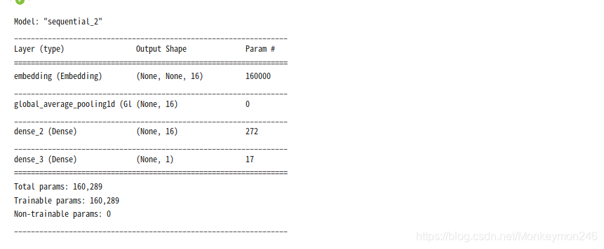
# 输入形状是用于电影评论的词汇数目（10,000 词）
vocab_size = 10000

model = keras.Sequential()
model.add(keras.layers.Embedding(vocab_size, 16))
model.add(keras.layers.GlobalAveragePooling1D())
model.add(keras.layers.Dense(16, activation='relu'))
model.add(keras.layers.Dense(1, activation='sigmoid'))

model.summary()

# 输入形状是用于电影评论的词汇数目（10,000 词）
vocab_size = 10000

model = keras.Sequential()
model.add(keras.layers.Embedding(vocab_size, 16))
model.add(keras.layers.GlobalAveragePooling1D())
model.add(keras.layers.Dense(16, activation='relu'))
model.add(keras.layers.Dense(1, activation='sigmoid'))

model.summary()

model.compile(optimizer='adam',
              loss='binary_crossentropy',
              metrics=['accuracy'])
x_val = train_data[:10000]
partial_x_train = train_data[10000:]

y_val = train_labels[:10000]
partial_y_train = train_labels[10000:]
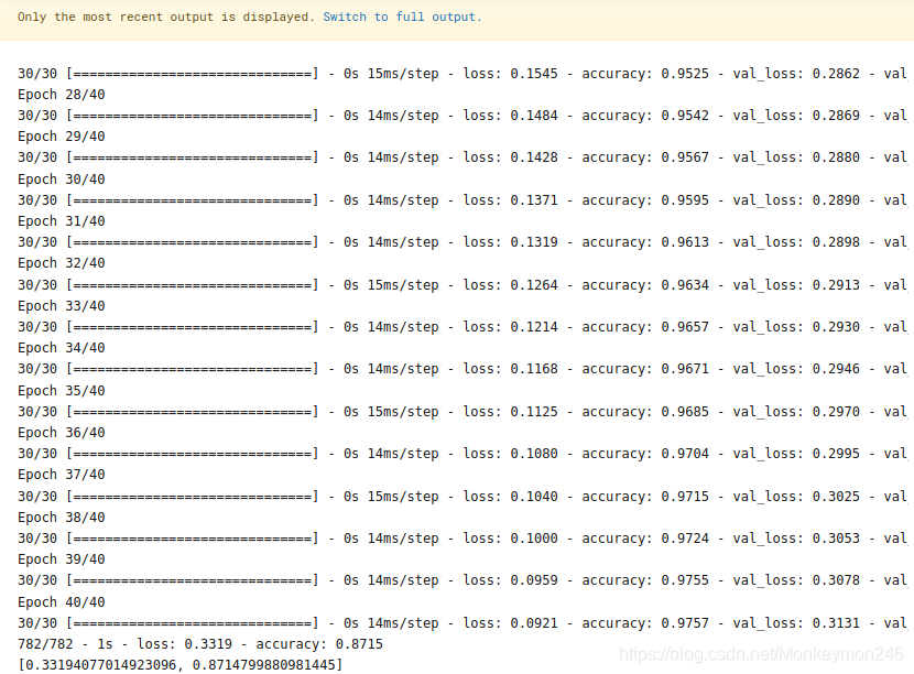
history = model.fit(partial_x_train,
                    partial_y_train,
                    epochs=40,
                    batch_size=512,
                    validation_data=(x_val, y_val),
                    verbose=1)
results = model.evaluate(test_data,  test_labels, verbose=2)

print(results)
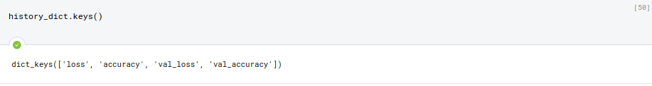
history_dict = history.history
history_dict.keys()
import matplotlib.pyplot as plt

acc = history_dict['accuracy']
val_acc = history_dict['val_accuracy']
loss = history_dict['loss']
val_loss = history_dict['val_loss']

epochs = range(1, len(acc) + 1)

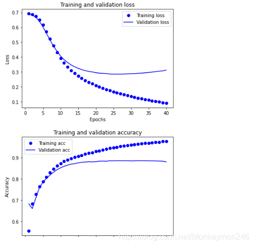
# “bo”代表 "蓝点"
plt.plot(epochs, loss, 'bo', label='Training loss')
# b代表“蓝色实线”
plt.plot(epochs, val_loss, 'b', label='Validation loss')
plt.title('Training and validation loss')
plt.xlabel('Epochs')
plt.ylabel('Loss')
plt.legend()

plt.show()
plt.clf()   # 清除数字

plt.plot(epochs, acc, 'bo', label='Training acc')
plt.plot(epochs, val_acc, 'b', label='Validation acc')
plt.title('Training and validation accuracy')
plt.xlabel('Epochs')
plt.ylabel('Accuracy')
plt.legend()

plt.show()

文本分类大概跑一下

validation_data=(x_val, y_val)验证集在这写

其中，history.history 该对象包含一个字典，其中包含训练阶段所发生的一切事件：

history_dict = history.history
history_dict.keys()

这个画loss的部分，可以学习下

Basic regression: Predict fuel efficiency

# 使用 seaborn 绘制矩阵图 (pairplot)
import pathlib

import matplotlib.pyplot as plt
import pandas as pd
import seaborn as sns

import tensorflow as tf

from tensorflow import keras
from tensorflow.keras import layers

print(tf.__version__)

dataset_path = keras.utils.get_file("auto-mpg.data", "http://archive.ics.uci.edu/ml/machine-learning-databases/auto-mpg/auto-mpg.data")
dataset_path

下载UCI的数据 keras.utils.get_file，路径都写好了

‘/home/jovyan/.keras/datasets/auto-mpg.data’

column_names = ['MPG','Cylinders','Displacement','Horsepower','Weight',
                'Acceleration', 'Model Year', 'Origin']
raw_dataset = pd.read_csv(dataset_path, names=column_names,
                      na_values = "?", comment='\t',
                      sep=" ", skipinitialspace=True)

dataset = raw_dataset.copy()
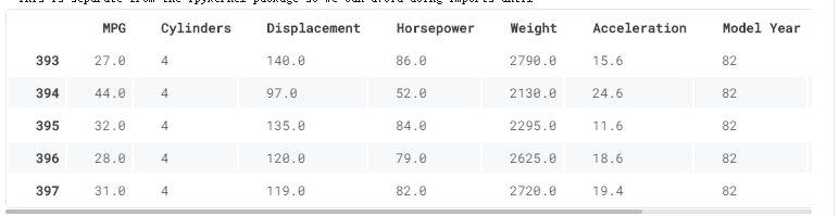
dataset.tail()

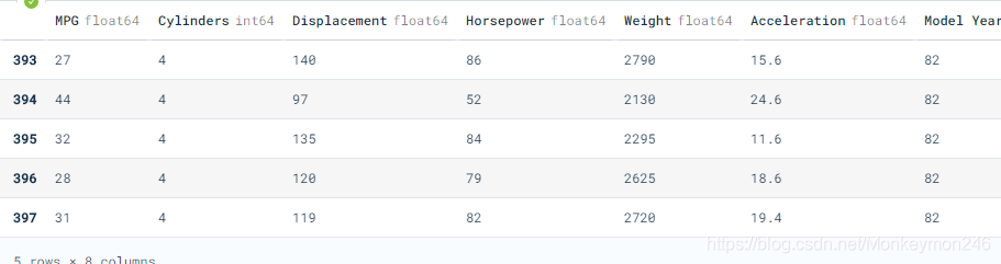
这个显示数据的方式太吊了：
dataset = raw_dataset.copy()
dataset.tail()

dataset.isna().sum()
dataset = dataset.dropna()
origin = dataset.pop('Origin')

snan判断是否nan（not a number）

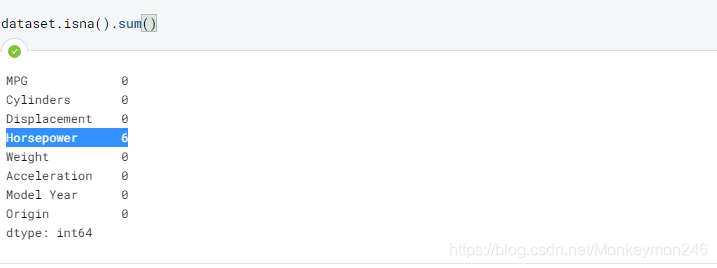
去掉之后，变成392 rows × 8 columns

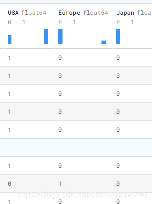
origin = dataset.pop('Origin')
dataset['USA'] = (origin == 1)*1.0
dataset['Europe'] = (origin == 2)*1.0
dataset['Japan'] = (origin == 3)*1.0
dataset.tail()

pop() 函数用于移除列表中的一个元素（默认最后一个元素），并且返回该元素的值。dataset[‘USA’]=392*1个数列，相当于赋值

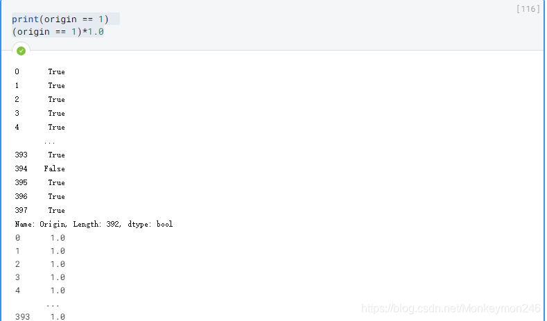
dataset后三列，one hot

train_dataset = dataset.sample(frac=0.8,random_state=0)
test_dataset = dataset.drop(train_dataset.index)

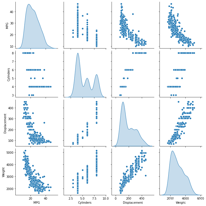
快速查看训练集中几对列的联合分布。
这个地方，太酷了

train_dataset = dataset.sample(frac=0.8,random_state=0)
test_dataset = dataset.drop(train_dataset.index)
sns.pairplot(train_dataset[["MPG", "Cylinders", "Displacement", "Weight"]], diag_kind="kde")

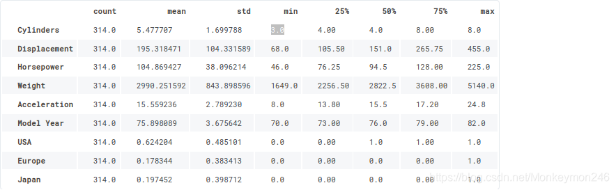
train_stats = train_dataset.describe()
train_stats.pop("MPG")
train_stats = train_stats.transpose()
train_stats

查看总体的数据统计: 数量，平均值，方差，最小值，递增到最大值

train_labels = train_dataset.pop('MPG')
test_labels = test_dataset.pop('MPG')

一个很好的递归手段，利用describe()

再次审视下上面的 train_stats 部分，并注意每个特征的范围有什么不同。

使用不同的尺度和范围对特征归一化是好的实践。尽管模型可能 在没有特征归一化的情况下收敛，它会使得模型训练更加复杂，并会造成生成的模型依赖输入所使用的单位选择。

注意：尽管我们仅仅从训练集中有意生成这些统计数据，但是这些统计信息也会用于归一化的测试数据集。我们需要这样做，将测试数据集放入到与已经训练过的模型相同的分布中。

def norm(x):
  return (x - train_stats['mean']) / train_stats['std']
normed_train_data = norm(train_dataset)
normed_test_data = norm(test_dataset)

模型是

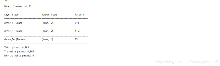
def build_model():
  model = keras.Sequential([
    layers.Dense(64, activation='relu', input_shape=[len(train_dataset.keys())]),
    layers.Dense(64, activation='relu'),
    layers.Dense(1)
  ])

  optimizer = tf.keras.optimizers.RMSprop(0.001)

  model.compile(loss='mse',
                optimizer=optimizer,
                metrics=['mae', 'mse'])
  return model

model = build_model()

model.summary()

example_batch = normed_train_data[:10]
example_result = model.predict(example_batch)
example_result

训练模型

对模型进行1000个周期的训练，并在 history 对象中记录训练和验证的准确性。

# 通过为每个完成的时期打印一个点来显示训练进度
class PrintDot(keras.callbacks.Callback):
  def on_epoch_end(self, epoch, logs):
    if epoch % 100 == 0: print('')
    print('.', end='')

EPOCHS = 1000

history = model.fit(
  normed_train_data, train_labels,
  epochs=EPOCHS, validation_split = 0.2, verbose=0,
  callbacks=[PrintDot()])

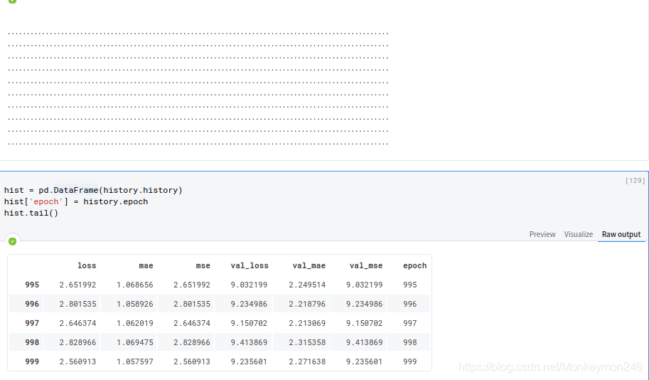
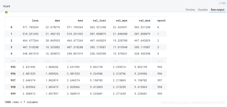
hist = pd.DataFrame(history.history)
hist['epoch'] = history.epoch
hist.tail()

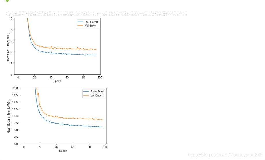
def plot_history(history):
  hist = pd.DataFrame(history.history)
  hist['epoch'] = history.epoch

  plt.figure()
  plt.xlabel('Epoch')
  plt.ylabel('Mean Abs Error [MPG]')
  plt.plot(hist['epoch'], hist['mae'],
           label='Train Error')
  plt.plot(hist['epoch'], hist['val_mae'],
           label = 'Val Error')
  plt.ylim([0,5])
  plt.legend()

  plt.figure()
  plt.xlabel('Epoch')
  plt.ylabel('Mean Square Error [$MPG^2$]')
  plt.plot(hist['epoch'], hist['mse'],
           label='Train Error')
  plt.plot(hist['epoch'], hist['val_mse'],
           label = 'Val Error')
  plt.ylim([0,20])
  plt.legend()
  plt.show()


plot_history(history)

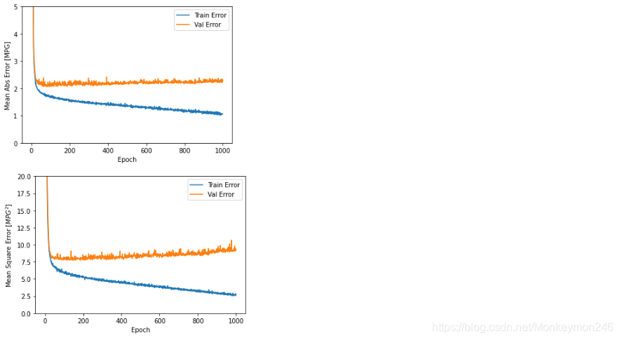
该图表显示在约100个 epochs 之后误差非但没有改进，反而出现恶化。 让我们更新 model.fit 调用，当验证值没有提高上是自动停止训练。 我们将使用一个 EarlyStopping callback 来测试每个 epoch 的训练条件。如果经过一定数量的 epochs 后没有改进，则自动停止训练。

model = build_model()

# patience 值用来检查改进 epochs 的数量
early_stop = keras.callbacks.EarlyStopping(monitor='val_loss', patience=10)

history = model.fit(normed_train_data, train_labels, epochs=EPOCHS,
                    validation_split = 0.2, verbose=0, callbacks=[early_stop, PrintDot()])

plot_history(history)

这个很好用啊，有木有，检测epochs 的数量

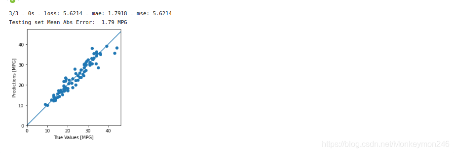
如图所示，验证集中的平均的误差通常在 +/- 2 MPG左右。 这个结果好么？ 我们将决定权留给你。

给我？

loss, mae, mse = model.evaluate(normed_test_data, test_labels, verbose=2)

print("Testing set Mean Abs Error: {:5.2f} MPG".format(mae))
test_predictions = model.predict(normed_test_data).flatten()

plt.scatter(test_labels, test_predictions)
plt.xlabel('True Values [MPG]')
plt.ylabel('Predictions [MPG]')
plt.axis('equal')
plt.axis('square')
plt.xlim([0,plt.xlim()[1]])
plt.ylim([0,plt.ylim()[1]])
_ = plt.plot([-100, 100], [-100, 100])

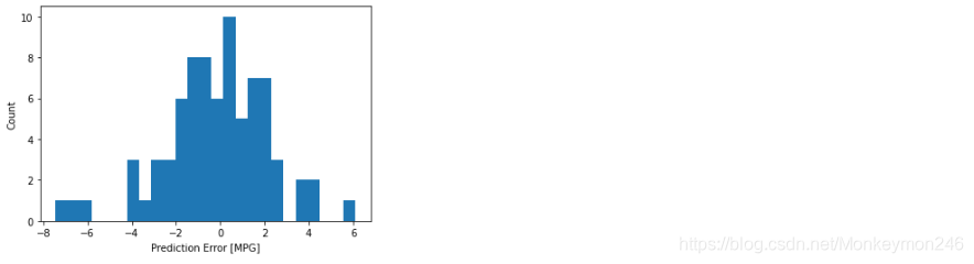
error = test_predictions - test_labels
plt.hist(error, bins = 25)
plt.xlabel("Prediction Error [MPG]")
_ = plt.ylabel("Count")

过拟合和欠拟合

过拟合好理解，欠拟合的意思是在训练集上还有提升的空间

import tensorflow as tf

from tensorflow.keras import layers
from tensorflow.keras import regularizers

print(tf.__version__)

!pip install -q git+https://github.com/tensorflow/docs

import tensorflow_docs as tfdocs
import tensorflow_docs.modeling
import tensorflow_docs.plots

from  IPython import display
from matplotlib import pyplot as plt

import numpy as np

import pathlib
import shutil
import tempfile

logdir = pathlib.Path(tempfile.mkdtemp())/"tensorboard_logs"
shutil.rmtree(logdir, ignore_errors=True)

The Higgs Dataset 包含11000000个示例，每个示例具有28个 features以及一个二进制类标签。

gz = tf.keras.utils.get_file('HIGGS.csv.gz', 'http://mlphysics.ics.uci.edu/data/higgs/HIGGS.csv.gz')

tf.data.experimental.CsvDataset类可用于直接从gzip文件读取csv记录，而无需中间的解压缩步骤。

FEATURES = 28
ds = tf.data.experimental.CsvDataset(gz,[float(),]*(FEATURES+1), compression_type="GZIP")

该csv阅读器类返回每个记录的标量列表。以下函数将该标量列表重新打包为（feature_vector，label）对。

def pack_row(*row):
  label = row[0]
  features = tf.stack(row[1:],1)
  return features, label

packed_ds = ds.batch(10000).map(pack_row).unbatch()

当处理大量数据时，TensorFlow效率最高。因此，与其单独重新打包每一行，不如创建一个新的数据集，该数据集采用10000个examples的批次，将pack_row函数应用于每个批次，然后将这些批次拆分回各个记录：packed_ds = ds.batch(10000).map(pack_row).unbatch()

——————————————————————————————————————————————————————————————
一些探索：

gz

‘/home/jovyan/.keras/datasets/HIGGS.csv.gz’

ds

<CsvDatasetV2 shapes: ((), (), (), (), (), (), (), (), (), (), (), (), (), (), (), (), (), (), (), (), (), (), (), (), (), (), (), (), ()), types: (tf.float32, tf.float32, tf.float32, tf.float32, tf.float32, tf.float32, tf.float32, tf.float32, tf.float32, tf.float32, tf.float32, tf.float32, tf.float32, tf.float32, tf.float32, tf.float32, tf.float32, tf.float32, tf.float32, tf.float32, tf.float32, tf.float32, tf.float32, tf.float32, tf.float32, tf.float32, tf.float32, tf.float32, tf.float32)>

ds.batch(10000)

<BatchDataset shapes: ((None,), (None,), (None,), (None,), (None,), (None,), (None,), (None,), (None,), (None,), (None,), (None,), (None,), (None,), (None,), (None,), (None,), (None,), (None,), (None,), (None,), (None,), (None,), (None,), (None,), (None,), (None,), (None,), (None,)), types: (tf.float32, tf.float32, tf.float32, tf.float32, tf.float32, tf.float32, tf.float32, tf.float32, tf.float32, tf.float32, tf.float32, tf.float32, tf.float32, tf.float32, tf.float32, tf.float32, tf.float32, tf.float32, tf.float32, tf.float32, tf.float32, tf.float32, tf.float32, tf.float32, tf.float32, tf.float32, tf.float32, tf.float32, tf.float32)>

ds.batch(10000).map(pack_row)

<MapDataset shapes: ((None, 28), (None,)), types: (tf.float32, tf.float32)>

ds.batch(10000).map(pack_row).unbatch()

<_UnbatchDataset shapes: ((28,), ()), types: (tf.float32, tf.float32)>

unbatch()将一个数据库分成多个元素
map()对每个数字进行处理

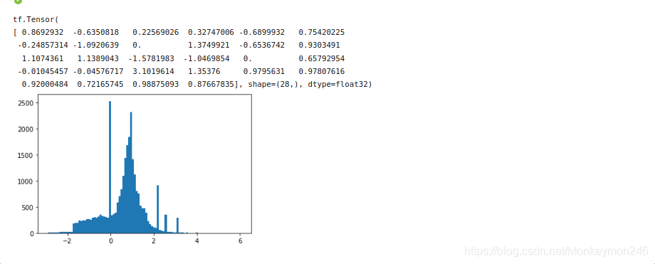
for features,label in packed_ds.batch(1000).take(1):
  print(features[0])
  plt.hist(features.numpy().flatten(), bins = 101)

为了使本教程相对较短，仅使用前1000个样本进行验证，然后使用10000个样本进行培训：

N_VALIDATION = int(1e3)
N_TRAIN = int(1e4)
BUFFER_SIZE = int(1e4)
BATCH_SIZE = 500
STEPS_PER_EPOCH = N_TRAIN//BATCH_SIZE
train_ds

这些数据集返回单个示例。使用.batch方法可创建适当大小的批次进行训练。批处理之前，记得.shuffle和.repeat训练集。

validate_ds = validate_ds.batch(BATCH_SIZE)
train_ds = train_ds.shuffle(BUFFER_SIZE).repeat().batch(BATCH_SIZE)

过拟合

逐渐降低学习率

lr_schedule = tf.keras.optimizers.schedules.InverseTimeDecay(
  0.001,
  decay_steps=STEPS_PER_EPOCH*1000,
  decay_rate=1,
  staircase=False)

def get_optimizer():
  return tf.keras.optimizers.Adam(lr_schedule)
step = np.linspace(0,100000)
lr = lr_schedule(step)
plt.figure(figsize = (8,6))
plt.plot(step/STEPS_PER_EPOCH, lr)
plt.ylim([0,max(plt.ylim())])
plt.xlabel('Epoch')
_ = plt.ylabel('Learning Rate')

上面的代码设置了一个schedules.InverseTimeDecay，以双曲线的方式将学习速率降低为1000周期时的基本速率的1 / 2、2000周期时的1/3等等。

接下来 用callbacks.EarlyStopping以避免冗长和不必要的培训时间。请注意，此回调设置为监视val_binary_crossentropy，而不是val_loss。这种差异稍后将变得很重要。

def get_callbacks(name):
  return [
    tfdocs.modeling.EpochDots(),
    tf.keras.callbacks.EarlyStopping(monitor='val_binary_crossentropy', patience=200),
    tf.keras.callbacks.TensorBoard(logdir/name),
  ]
def compile_and_fit(model, name, optimizer=None, max_epochs=10000):
  if optimizer is None:
    optimizer = get_optimizer()
  model.compile(optimizer=optimizer,
                loss=tf.keras.losses.BinaryCrossentropy(from_logits=True),
                metrics=[
                  tf.keras.losses.BinaryCrossentropy(
                      from_logits=True, name='binary_crossentropy'),
                  'accuracy'])

  model.summary()

  history = model.fit(
    train_ds,
    steps_per_epoch = STEPS_PER_EPOCH,
    epochs=max_epochs,
    validation_data=validate_ds,
    callbacks=get_callbacks(name),
    verbose=0)
  return history
  
tiny_model = tf.keras.Sequential([
    layers.Dense(16, activation='elu', input_shape=(FEATURES,)),
    layers.Dense(1)
])

size_histories = {}

size_histories['Tiny'] = compile_and_fit(tiny_model, 'sizes/Tiny')

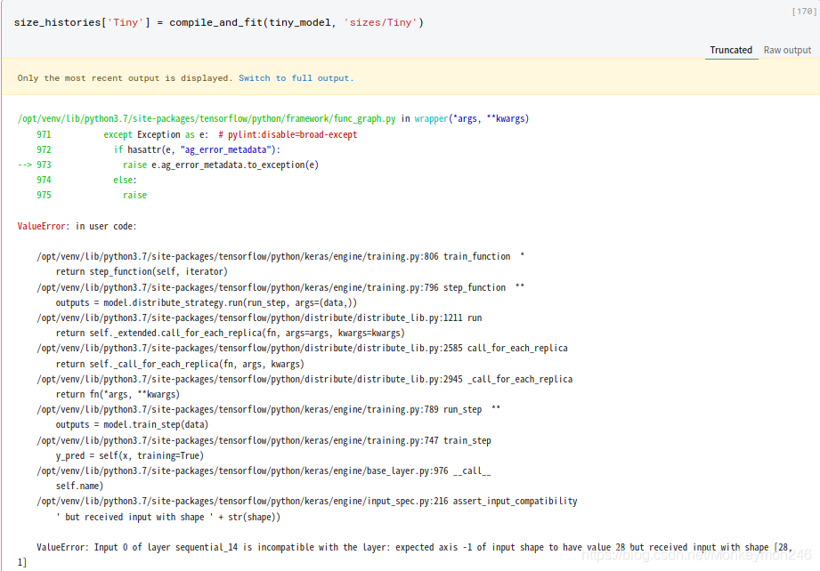
结果报错
原因出在这句

size_histories['Tiny'] = compile_and_fit(tiny_model, 'sizes/Tiny')