如果对Tensorflow实现最新的Yolo v7算法有兴趣的朋友,可以参见我最新发布的文章, Yolo v7的最简TensorFlow实现_gzroy的博客-CSDN博客
YOLO是一个非常出名的目标检测的模型,兼具精度和性能,在工业界的应用非常广泛。我司也是运用了YOLO V3算法在智能制造领域,用于协助机械臂进行精确定位。不过可惜YOLO的原作者自从推出了V3算法之后,因为个人的理念,不希望计算机视觉技术用在军事等领域上,宣布不再从事这方面的研究。所幸Alexey Bochkovskiy一直持续研究YOLO算法,并在2020年发布了论文,提出了V4版本,作出了很多改进,融合了在目标检测,图像识别方面的很多研究成果,实现了进一步的提升。具体可以参阅相关的论文。
这里我尝试基于Tensorflow 2.x版本来重现YOLO v4,希望可以加深对YOLO算法的理解。
Imagenet的预训练
网络结构
Darknet的csdarknet53-omega.cfg文件对应的是以CSPDarknet53为网络结构,对Imagenet的数据集进行图像分类。预训练后的模型可以作为目标检测的骨干网络。
首先我用Tensorflow来搭建这个CSPDarknet53的网络。可以用netron.app这个网站,打开cfg文件,即可显示这个网络结构的详细信息,按照这个架构来搭建网络,以下是这个网络结构的其中一部分的截图:
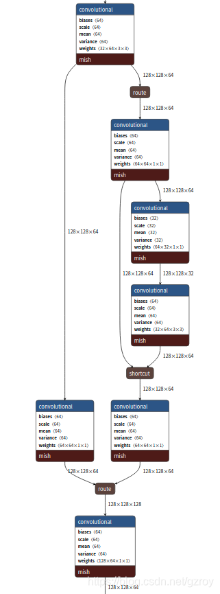
tensorflow的代码如下:
import tensorflow as tf
import tensorflow_addons as tfa
from tensorflow.keras import Model
l=tf.keras.layers

def _conv(inputs, filters, kernel_size, strides, bias=True, normalize=True, activation='mish'):
    output = inputs
    padding_str = 'same'
    output = l.Conv2D(filters, kernel_size, strides, padding_str, \
                  'channels_first', use_bias=bias, \
                  kernel_initializer='he_normal')(output)
    if normalize:
        output = l.BatchNormalization(axis=1)(output)
    if activation=='leaky':
        output = l.LeakyReLU(alpha=0.1)(output)
    elif activation=='mish':
        output = tfa.activations.mish(output)
    else:
        output = output
    return output

def _csp_1(inputs, filters, block_num, activation='mish', name=None):
    output = _conv(inputs, filters*2, 3, 2)
    output_1 = _conv(output, filters*2, 1, 1)
    output = _conv(output,filters*2, 1, 1)
    for i in range(block_num):
        output_2 = _conv(output, filters, 1, 1)
        output_2 = _conv(output_2, filters*2, 3, 1)
        output_2 = l.Add()([output_2, output])
        output = output_2
    output_2 = _conv(output_2,filters*2, 1, 1)
    output = l.Concatenate(axis=1)([output_1, output_2])
    output = _conv(output, filters*2, 1, 1)
    return output

def _csp_2(inputs, filters, block_num, training=True, activation='mish', name=None):
    output = _conv(inputs, filters*2, 3, 2)
    output_1 = _conv(output, filters, 1, 1)
    output = _conv(output,filters, 1, 1)
    for i in range(block_num):
        output_2 = _conv(output,filters, 1, 1)
        output_2 = _conv(output_2, filters, 3, 1)
        output_2 = l.Add()([output_2, output])
        #output_3 = _conv(output_2, filters, 1, 1)
        #output_3 = _conv(output_3, filters, 3, 1)
        #output_3 = l.Add()([output_2, output_3])
        output = output_2
    #output_3 = _conv(output_3,filters, 1, 1,)
    output_2 = _conv(output_2,filters, 1, 1,)
    output = l.Concatenate(axis=1)([output_1, output_2])
    output = _conv(output, filters*2, 1, 1)
    return output

def CSPDarknet53_model():
    image = tf.keras.Input(shape=(3,None,None))    # 3*H*W
    net = _conv(image, 32, 3, 1)    #32*H*W
    net = _csp_1(net, 32, 1)        #64*H/2*W/2
    net = _csp_2(net, 64, 2)        #128*H/4*W/4
    net = _csp_2(net, 128, 8)       #256*H/8*W/8
    route1 = l.Activation('linear', dtype='float32', name='route1')(net)   #256*H/8*W/8
    net = _csp_2(net, 256, 8)       #512*H/16*W/16
    route2 = l.Activation('linear', dtype='float32', name='route2')(net)   #512*H/16*W/16
    net = _csp_2(net, 512, 4)       #1024*H/32*W/32
    route3 = l.Activation('linear', dtype='float32', name='route3')(net)   #1024*H/32*W/32
    net = tf.reduce_mean(net, axis=[2,3], keepdims=True)
    net = _conv(net, 1000, 1, 1, True, False, 'linear')
    net = l.Flatten(data_format='channels_first', name='logits')(net)
    net = l.Activation('linear', dtype='float32', name='output')(net)
    model = tf.keras.Model(inputs=image, outputs=[net, route1, route2, route3])
    return model
在这个网络里面有三个层route1, route2, route3是用来输出不同维度的图形特征值,给以后搭建目标检测网络的时候来用。在Imagenet的分类训练中先用不到。
数据预处理
在cfg文件里面设置了采用cutmix和mosaic这两种方式,查看darknet的源代码,在data.c的load_data_augment函数里面定义了这两种方式的处理。简单来说,cutmix是组合两张图片,在其中一张图片里面随即定义一个矩形区域,填充第二张图片的内容。mosaic是组合4张图片,随即划分四个区域,分别填充这四张图片的内容。
用tensorflow来实现这个机制,我的做法是这样的,首先在dataset的map操作中对单张图片进行缩放,反转,改变图像饱和度等操作,然后通过要用到dataset.window,指定window的大小为4,表示每次取四张图片,然后通过flatmap来把四张图片组合成一个Tensor,然后再对这个Tensor来随机进行cutmix或者mosaic的操作。
Imagenet数据集的准备
需要准备Imagenet的数据,具体可以见我以前的另一篇博客,基于Tensorflow的Imagenet数据集的完整处理过程(包括物体标识框BBOX的处理)_valid_classes_gzroy的博客-CSDN博客
单张图片的变换
对单张图片的变换主要包括以下步骤,假设图片的原始尺寸为600*400:
- 随机缩放图像的宽(缩放比例为0.75-1/0.75,例如0.8),计算宽和高的短边。宽为600*0.8=480, 高为400,短边为400
- 随机确定一个正方形图像的边长(范围为128-448,例如300),并计算这个边长和第一步得到的短边的长度的比值,300/400=0.75
- 根据比值计算需要缩放的图像的宽和高,宽为400*0.75=300, 高为600*0.8*0.75=360,并缩放图像到这个尺寸
- 假设我们最终要获取的图像大小为256*256, 如果第3步的图像的短边比这个图像的边长256小,计算其比值,并缩放图像到这个大小。因为第3步我们得到的图像的短边是300,比256大,不需要作缩放。
- 随机剪切第4步的图像,获取一个256*256的区域。
- 随机翻转图像
- 随机旋转图像,旋转角度为-7到7度之间的一个随机值
- 随机调整图片的hue, 饱和度,明亮度,调整系数是在[0.6, 1.4]之间的一个随机值
- 给图片添加PCA噪音,其系数为高斯分布(0,0.1)的一个随机值
- 标准化图片的RGB的值,给RGB 3个Channel分别减去123.68,116.779,103.939,然后再除以58.393,57.12,57.375
代码如下:
imageWidth = 256
imageHeight = 256
min_crop=128
max_crop=448
random_min_aspect = 0.75
random_max_aspect = 1/0.75
random_angle = 7.
eigvec = tf.constant([
    [-0.5675, 0.7192, 0.4009],
    [-0.5808, -0.0045, -0.8140],
    [-0.5836, -0.6948, 0.4203]],
    shape=[3,3], dtype=tf.float32
)
eigval = tf.constant([55.46, 4.794, 1.148], shape=[3,1], dtype=tf.float32)
mean_RGB = tf.constant([123.68, 116.779, 109.939], dtype=tf.float32)
std_RGB = tf.constant([58.393, 57.12, 57.375], dtype=tf.float32)

# Parse TFRECORD and distort the image for train
def _parse_function(example_proto):
    features = {
        "image": tf.io.FixedLenFeature([], tf.string, default_value=""),
        "height": tf.io.FixedLenFeature([1], tf.int64, default_value=[0]),
        "width": tf.io.FixedLenFeature([1], tf.int64, default_value=[0]),
        "channels": tf.io.FixedLenFeature([1], tf.int64, default_value=[3]),
        "colorspace": tf.io.FixedLenFeature([], tf.string, default_value=""),
        "img_format": tf.io.FixedLenFeature([], tf.string, default_value=""),
        "label": tf.io.FixedLenFeature([1], tf.int64, default_value=[0]),
        "bbox_xmin": tf.io.VarLenFeature(tf.float32),
        "bbox_xmax": tf.io.VarLenFeature(tf.float32),
        "bbox_ymin": tf.io.VarLenFeature(tf.float32),
        "bbox_ymax": tf.io.VarLenFeature(tf.float32),
        "text": tf.io.FixedLenFeature([], tf.string, default_value=""),
        "filename": tf.io.FixedLenFeature([], tf.string, default_value="")
    }
    parsed_features = tf.io.parse_single_example(example_proto, features)
    image_decoded = tf.image.decode_jpeg(parsed_features["image"], channels=3)
    image_decoded = tf.cast(image_decoded, dtype=tf.float32)

    # Random crop the image
    shape = tf.shape(image_decoded)
    height, width = shape[0], shape[1]
    random_aspect = tf.random.uniform(shape=[], minval=random_min_aspect, maxval=random_max_aspect)
    random_size = tf.random.uniform(shape=[], minval=min_crop, maxval=max_crop, dtype=tf.int32)
    min = tf.cond(
        height<tf.cast(tf.cast(width, tf.float32)*random_aspect, tf.int32),
        lambda:height,
        lambda:tf.cast(tf.cast(width, tf.float32)*random_aspect, tf.int32))
    scale = tf.cast(random_size/min, tf.float32)
    crop_height = tf.cast(tf.cast(height, tf.float32)*scale, tf.int32)
    crop_width = tf.cast(tf.cast(width, tf.float32)*random_aspect*scale, tf.int32)
    crop_resized = tf.image.resize(image_decoded, [crop_height, crop_width])
    min = tf.cond(crop_height<crop_width, lambda:crop_height, lambda:crop_width)
    ratio = tf.cond(min<random_size, lambda:tf.cast(random_size/min, tf.float32), lambda:1.)
    scale = tf.cond(random_size<imageHeight, lambda:tf.cast(imageHeight/random_size, tf.float32), lambda:1.)
    resized = tf.image.resize(
        crop_resized,
        [
            tf.cast(tf.cast(crop_height, tf.float32)*ratio*scale, tf.int32)+1,
            tf.cast(tf.cast(crop_width, tf.float32)*ratio*scale, tf.int32)+1
        ]
    )
    cropped = tf.image.random_crop(resized, [imageHeight, imageWidth, 3])

    # Flip to add a little more random distortion in.
    flipped = tf.image.random_flip_left_right(cropped)

    # Random rotate the image
    angle = tf.random.uniform(shape=[], minval=-random_angle, maxval=random_angle)*np.pi/180
    rotated = tfa.image.rotate(flipped, angle)

    # Random distort the image
    distorted = tf.image.random_hue(rotated, max_delta=0.3)
    distorted = tf.image.random_saturation(distorted, lower=0.6, upper=1.4)
    distorted = tf.image.random_brightness(distorted, max_delta=0.3)

    # Add PCA noice
    alpha = tf.random.normal([3], mean=0.0, stddev=0.1)
    pca_noice = tf.reshape(tf.matmul(tf.multiply(eigvec,alpha), eigval), [3])
    distorted = tf.add(distorted, pca_noice)

    # Normalize RGB
    distorted = tf.subtract(distorted, mean_RGB)
    distorted = tf.divide(distorted, std_RGB)

    image_train = tf.transpose(distorted, perm=[2, 0, 1])
    features = {'input_1': image_train}
    labels = tf.one_hot(parsed_features["label"][0], depth=1000)

    return features, labels
多张图片的变换
之后就是对多张图片进行cutmix或者mosaic的操作。首先定义一个_flatmap_function,用于把4张图片组合为一个batch。然后定义一个_mixup_function,随机进行以下操作
- 50%的机率返回其中的一张图片
- 25%的机率对其中的两张图片进行cutmix操作,组合为一张新的图片并返回
- 25%的机率对4张图片进行mosaic操作,组合为一张新的图片并返回
代码如下:
def _flatmap_function(features):
    dataset_image = features['image'].padded_batch(4, [3, imageHeight, imageWidth], drop_remainder=True)
    dataset_label = features['label'].padded_batch(4, [1000], drop_remainder=True)
    dataset_combined = tf.data.Dataset.zip({'image':dataset_image, 'label':dataset_label})
    return dataset_combined

def _mixup_function(features):
    images = features['image']
    labels = features['label']

    def _cutmix():
        min = 0.3
        max = 0.8
        cut_w = tf.random.uniform(shape=[], minval=int(min*imageWidth), maxval=int(max*imageWidth), dtype=tf.int32)
        cut_h = tf.random.uniform(shape=[], minval=int(min*imageHeight), maxval=int(max*imageHeight), dtype=tf.int32)
        cut_x = tf.random.uniform(shape=[], minval=0, maxval=(imageWidth-cut_w-1), dtype=tf.int32)
        cut_y = tf.random.uniform(shape=[], minval=0, maxval=(imageHeight-cut_h-1), dtype=tf.int32)
        left = cut_x
        right = cut_x+cut_w
        top = cut_y
        bottom = cut_y+cut_h
        alpha = tf.cast(cut_w*cut_h/(imageWidth*imageHeight), tf.float32)
        beta = tf.cast(1.-alpha, tf.float32)
        img0 = images[0]
        img1 = images[1]
        image = tf.concat([
            img0[:,:top,:],
            tf.concat([img0[:,top:bottom,:left], img1[:,top:bottom,left:right], img0[:,top:bottom,right:]], axis=-1),
            img0[:,bottom:,:]
        ], axis=-2)
        label0 = labels[0]
        label1 = labels[1]
        label = label0*beta+label1*alpha
        return image, label

    def _mosaic():
        area = imageWidth*imageHeight
        min_offset = 0.2
        cut_x = tf.random.uniform(shape=[], minval=int(min_offset*imageWidth),  maxval=int((1-min_offset)*imageWidth), dtype=tf.int32)
        cut_y = tf.random.uniform(shape=[], minval=int(min_offset*imageHeight), maxval=int((1-min_offset)*imageHeight), dtype=tf.int32)
        ratio_0 = tf.cast(cut_x*cut_y/area, tf.float32)
        ratio_1 = tf.cast((imageWidth-cut_x)*cut_y/area, tf.float32)
        ratio_2 = tf.cast((imageHeight-cut_y)*cut_x/area, tf.float32)
        ratio_3 = tf.cast((imageHeight-cut_y)*(imageWidth-cut_x)/area, tf.float32)
        img0 = images[0]
        img1 = images[1]
        img2 = images[2]
        img3 = images[3]
        image = tf.concat([
            tf.concat([
                img0[:,(imageHeight-cut_y)//2:((imageHeight-cut_y)//2+cut_y),(imageWidth-cut_x)//2:((imageWidth-cut_x)//2+cut_x)],
                img1[:,(imageHeight-cut_y)//2:((imageHeight-cut_y)//2+cut_y),cut_x//2:(cut_x//2+imageWidth-cut_x)]
            ], axis=-1),
            tf.concat([
                img2[:,cut_y//2:(cut_y//2+imageHeight-cut_y),(imageWidth-cut_x)//2:((imageWidth-cut_x)//2+cut_x)],
                img3[:,cut_y//2:(cut_y//2+imageHeight-cut_y),cut_x//2:(cut_x//2+imageWidth-cut_x)]
            ], axis=-1)
        ], axis=-2)
        label = labels[0]*ratio_0+labels[1]*ratio_1+labels[2]*ratio_2+labels[3]*ratio_3
        return image, label

    def _mix_random():
        flag = tf.random.uniform(shape=[], minval=0., maxval=1.)
        image, label = tf.cond(tf.less(flag, 0.5), _cutmix, _mosaic)
        return image, label

    flag = tf.random.uniform(shape=[], minval=0., maxval=1.)
    image, label = tf.cond(
        tf.less(flag, 0.5),
        lambda:(images[0],labels[0]),
        _mix_random
    )
    return image, label
构建训练集dataset
最后我们就可以构建一个dataset,完成整个对图片的预处理过程,生成训练集数据
def train_input_fn():
    dataset_train = tf.data.TFRecordDataset(train_files)
    dataset_train = dataset_train.map(_parse_function, num_parallel_calls=tf.data.experimental.AUTOTUNE)
    dataset_train = dataset_train.window(4)
    dataset_train = dataset_train.flat_map(_flatmap_function)
    dataset_train = dataset_train.map(_mixup_function, num_parallel_calls=tf.data.experimental.AUTOTUNE)
    dataset_train = dataset_train.shuffle(buffer_size=1600, reshuffle_each_iteration=True)
    dataset_train = dataset_train.repeat(10)
    dataset_train = dataset_train.batch(batch_size)
    dataset_train = dataset_train.prefetch(batch_size)
    return dataset_train
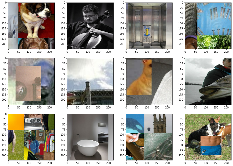
以下是生成的训练集的图片的示例,包括了cutmix和mosaic。
构建测试集dataset
测试集的构建就相对简单,只需要把单张图像缩放裁减即可。
def _parse_test_function(example_proto):
    features = {
        "image": tf.io.FixedLenFeature([], tf.string, default_value=""),
        "height": tf.io.FixedLenFeature([1], tf.int64, default_value=[0]),
        "width": tf.io.FixedLenFeature([1], tf.int64, default_value=[0]),
        "channels": tf.io.FixedLenFeature([1], tf.int64, default_value=[3]),
        "colorspace": tf.io.FixedLenFeature([], tf.string, default_value=""),
        "img_format": tf.io.FixedLenFeature([], tf.string, default_value=""),
        "label": tf.io.FixedLenFeature([1], tf.int64, default_value=[0]),
        "bbox_xmin": tf.io.VarLenFeature(tf.float32),
        "bbox_xmax": tf.io.VarLenFeature(tf.float32),
        "bbox_ymin": tf.io.VarLenFeature(tf.float32),
        "bbox_ymax": tf.io.VarLenFeature(tf.float32),
        "text": tf.io.FixedLenFeature([], tf.string, default_value=""),
        "filename": tf.io.FixedLenFeature([], tf.string, default_value="")
    }
    parsed_features = tf.io.parse_single_example(example_proto, features)
    image_decoded = tf.image.decode_jpeg(parsed_features["image"], channels=3)
    image_decoded = tf.cast(image_decoded, dtype=tf.float32)
    shape = tf.shape(image_decoded)
    height, width = shape[0], shape[1]
    resized_height, resized_width = tf.cond(height<width,
        lambda: (tf.cast(tf.multiply(tf.cast(height, tf.float64),tf.divide(imageWidth,width)), tf.int32), imageWidth),
        lambda: (imageHeight, tf.cast(tf.multiply(tf.cast(width, tf.float64),tf.divide(imageHeight,height)), tf.int32))
    )
    padded_height = imageHeight - resized_height
    padded_width = imageWidth - resized_width
    image_resized = tf.image.resize(image_decoded, [resized_height, resized_width])
    image_padded = tf.image.pad_to_bounding_box(image_resized, padded_height//2, padded_width//2, imageHeight, imageWidth)
    # Normalize RGB
    image_valid = tf.subtract(image_padded, mean_RGB)
    image_valid = tf.divide(image_valid, std_RGB)
    image_valid = tf.transpose(image_valid, perm=[2, 0, 1])
    features = {'input_1': image_valid}
    labels = tf.one_hot(parsed_features["label"][0], depth=1000)
    return features, labels

def val_input_fn():
    dataset_valid = tf.data.TFRecordDataset(valid_files)
    dataset_valid = dataset_valid.map(_parse_test_function, num_parallel_calls=tf.data.experimental.AUTOTUNE)
    dataset_valid = dataset_valid.take(100000)
    dataset_valid = dataset_valid.batch(batch_size)
    dataset_valid = dataset_valid.prefetch(batch_size)
    return dataset_valid
训练模型
现在我们可以编写代码来对模型进行训练了,这里的学习率的变化也是参考darknet的实现,采用指数衰减的方式。Darknet里面每个Batch是128,初始学习率是0.1,我的电脑显卡是2080Ti,显存是11G,在混合精度下每个Batch最大值是64,因此初始学习率也减半调整为0.05。代码如下:
initial_warmup_steps = 1000
initial_lr = 0.05
maximum_batches = 2400000
power = 4

START_EPOCH = 0
NUM_EPOCH = 1
STEPS_EPOCH = 20000
STEPS_OFFSET = 0
with tf.device('/GPU:0'):
    model = CSPDarknet53_model()
    optimizer=tf.keras.optimizers.SGD(learning_rate=0.0001, momentum=0.9)
    # If load model from previous, uncomment the below two line
    #tfa.register_all()
    #model = tf.keras.models.load_model('models/darknet53_custom_training_5000.h5')
    @tf.function
    def train_step(inputs, labels):
        with tf.GradientTape() as tape:
            predictions = model(inputs, training=True)
            pred_loss = tf.keras.losses.CategoricalCrossentropy(from_logits=True, label_smoothing=0.1)(labels, predictions[0])
            total_loss = pred_loss
        gradients = tape.gradient(total_loss, model.trainable_variables)
        optimizer.apply_gradients(zip(gradients, model.trainable_variables))
        return total_loss

    for epoch in range(NUM_EPOCH):
        start_step = tf.keras.backend.get_value(optimizer.iterations)+STEPS_OFFSET
        steps = start_step
        loss_sum = 0
        start_time = time.time()
        for inputs, labels in train_data:
            if (steps-start_step)>STEPS_EPOCH:
                break
            loss_sum += train_step(inputs, labels)
            steps = tf.keras.backend.get_value(optimizer.iterations)+STEPS_OFFSET
            if steps <= initial_warmup_steps:
                lr = initial_lr * math.pow(steps/initial_warmup_steps, power)
                tf.keras.backend.set_value(optimizer.lr, lr)
            else:
                lr = initial_lr * math.pow((1.-steps/maximum_batches), power)
                tf.keras.backend.set_value(optimizer.lr, lr)
            if steps%100 == 0:
                elasp_time = time.time()-start_time
                print("Step:{}, Loss:{:4.2f}, LR:{:5f}, Time:{:3.1f}s".format(steps, loss_sum/100, lr, elasp_time))
                loss_sum = 0
                start_time = time.time()
            steps += 1
        model.save('models/CSPDarknet53_original_'+str(START_EPOCH+epoch)+'.h5')
        m1 = tf.keras.metrics.CategoricalAccuracy()
        m2 = tf.keras.metrics.TopKCategoricalAccuracy()
        for inputs, labels in val_data:
            val_predict_logits = model(inputs, training=False)[0]
            val_predict = tf.keras.activations.softmax(val_predict_logits)
            m1.update_state(labels, val_predict)
            m2.update_state(labels, val_predict)
        print("Top-1 Accuracy:%f, Top-5 Accuracy:%f"%(m1.result().numpy(),m2.result().numpy()))
        m1.reset_states()
        m2.reset_states()
模型训练了大概30个EPOCH,TOP-5的准确率为90%,TOP-1的准确度为75%
YOLO的训练
在完成了Imagenet的预训练之后,我们就可以开始进行YOLO模型的搭建和训练了
YOLO模型的搭建
同样我们可以用netron.app这个网站来查看darknet里面关于yolo v4的网络结构,对应的文件是yolov4.cfg。下图是YOLO网络的一部分的截图
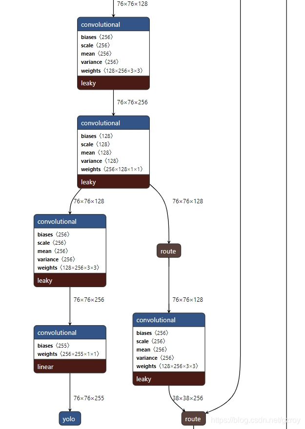
YOLO模型的输入是之前我们ImageNet预训练里面用到的CSPDarknet_model的三个输出,模型的输出是对应三个不同尺度的物体检测结果。假设我们的输入图形是512*512,那么对应的三个检测尺度分别是512/8=64, 512/16=32, 512/32=8。输出的向量的维度是[batch_size, 3*(1+4+80), 64*64+32*32+8*8]。这里面的3*(1+4+80)=255的维度对应的是每个检测尺度有3个不同尺寸的Anchor box,每个box的预测值是(1+4+80), 其中1表示是预测物体是否存在,4表示物体的中心点的坐标xy以及宽和高,80表示对应COCO 80个物体类别。代码如下:
def YOLO_model():
    route1 = tf.keras.Input(shape=(256,None,None), name='input1')        #256*H/8*W/8
    route2 = tf.keras.Input(shape=(512,None,None), name='input2')        #512*H/16*W/16
    route3 = tf.keras.Input(shape=(1024,None,None), name='input3')       #1024*H/32*W/32
    output1 = _conv(route1, 128, 1, 1, activation='leaky')               #128*H/8*W/8
    output2 = _conv(route2, 256, 1, 1, activation='leaky')               #256*H/16*W/16
    output3 = _conv(route3, 512, 1, 1, activation='leaky')               #512*H/32*W/32
    output3 = _conv(output3, 1024, 3, 1, activation='leaky')             #1024*H/32*W/32
    output3 = _conv(output3, 512, 1, 1, activation='leaky')              #512*H/32*W/32
    spp1 = l.MaxPooling2D(pool_size=(5, 5), strides=(1, 1), padding='same', data_format='channels_first')(output3)
    spp2 = l.MaxPooling2D(pool_size=(9, 9), strides=(1, 1), padding='same', data_format='channels_first')(output3)
    spp3 = l.MaxPooling2D(pool_size=(13, 13), strides=(1, 1), padding='same', data_format='channels_first')(output3)
    output3 = l.Concatenate(axis=1)([spp1, spp2, spp3, output3])         #2048*H/32*W/32
    output3 = _conv(output3, 512, 1, 1, activation='leaky')              #512*H/32*W/32
    output3 = _conv(output3, 1024, 3, 1, activation='leaky')             #1024*H/32*W/32
    output3 = _conv(output3, 512, 1, 1, activation='leaky')              #512*H/32*W/32
    output4 = _conv(output3, 256, 1, 1, activation='leaky')              #256*H/32*W/32
    output4 = l.UpSampling2D((2,2),"channels_first",'nearest')(output4)  #256*H/16*W/16
    output4 = l.Concatenate(axis=1)([output2, output4])                  #512*H/16*W/16
    output4 = _conv(output4, 256, 1, 1, activation='leaky')              #256*H/16*W/16
    output4 = _conv(output4, 512, 3, 1, activation='leaky')              #512*H/16*W/16
    output4 = _conv(output4, 256, 1, 1, activation='leaky')              #256*H/16*W/16
    output4 = _conv(output4, 512, 3, 1, activation='leaky')              #512*H/16*W/16
    output4 = _conv(output4, 256, 1, 1, activation='leaky')              #256*H/16*W/16
    output5 = _conv(output4, 128, 1, 1, activation='leaky')              #128*H/16*W/16
    output5 = l.UpSampling2D((2,2),"channels_first",'nearest')(output5)  #128*H/8*W/8
    output5 = l.Concatenate(axis=1)([output1, output5])                  #256*H/8*W/8
    output5 = _conv(output5, 128, 1, 1, activation='leaky')              #128*H/8*W/8
    output5 = _conv(output5, 256, 3, 1, activation='leaky')              #256*H/8*W/8
    output5 = _conv(output5, 128, 1, 1, activation='leaky')              #128*H/8*W/8
    output5 = _conv(output5, 256, 3, 1, activation='leaky')              #256*H/8*W/8
    output5 = _conv(output5, 128, 1, 1, activation='leaky')              #128*H/8*W/8
    yolo_small = _conv(output5, 256, 3, 1, activation='leaky')           #256*H/8*W/8
    yolo_small = _conv(yolo_small, 255, 1, 1, normalize=False, activation='linear')       #255*H/8*W/8
    yolo_small = l.Activation('linear', dtype='float32', name='yolo_small')(yolo_small)   #256*H/8*W/8
    yolo_small = l.Reshape((255, -1))(yolo_small)
    output5 = _conv(output5, 256, 3, 2, activation='leaky')              #256*H/16*W/16
    output6 = l.Concatenate(axis=1)([output4, output5])                  #512*H/16*W/16
    output6 = _conv(output6, 256, 1, 1, activation='leaky')              #256*H/16*W/16
    output6 = _conv(output6, 512, 3, 1, activation='leaky')              #512*H/16*W/16
    output6 = _conv(output6, 256, 1, 1, activation='leaky')              #256*H/16*W/16
    output6 = _conv(output6, 512, 3, 1, activation='leaky')              #512*H/16*W/16
    output6 = _conv(output6, 256, 1, 1, activation='leaky')              #256*H/16*W/16
    yolo_medium = _conv(output6, 512, 3, 1, activation='leaky')          #512*H/16*W/16
    yolo_medium = _conv(yolo_medium, 255, 1, 1, normalize=False, activation='linear')  #255*H/16*W/16
    yolo_medium = l.Activation('linear', dtype='float32', name='yolo_medium')(yolo_medium)
    yolo_medium = l.Reshape((255, -1))(yolo_medium)
    output6 = _conv(output6, 512, 3, 2, activation='leaky')              #512*H/32*W/32
    output6 = l.Concatenate(axis=1)([output3, output6])                  #1024*H/32*W/32
    output6 = _conv(output6, 512, 1, 1, activation='leaky')              #512*H/32*W/32
    output6 = _conv(output6, 1024, 3, 1, activation='leaky')             #1024*H/32*W/32
    output6 = _conv(output6, 512, 1, 1, activation='leaky')              #512*H/32*W/32
    output6 = _conv(output6, 1024, 3, 1, activation='leaky')             #1024*H/32*W/32
    output6 = _conv(output6, 512, 1, 1, activation='leaky')              #512*H/32*W/32
    output6 = _conv(output6, 1024, 3, 1, activation='leaky')             #1024*H/32*W/32
    yolo_big = _conv(output6, 255, 1, 1, normalize=False, activation='linear')  #255*H/32*W/32
    yolo_big = l.Activation('linear', dtype='float32', name='yolo_big')(yolo_big)
    yolo_big = l.Reshape((255, -1))(yolo_big)
    yolo = l.Concatenate(axis=-1)([yolo_small, yolo_medium, yolo_big])
    yolo = tf.transpose(yolo, perm=[0, 2, 1])
    yolo = l.Activation('linear', dtype='float32')(yolo)
    model = tf.keras.Model(inputs=[route1, route2, route3], outputs=yolo, name='yolo')
    return model
数据预处理
这里是用COCO的数据来进行训练和预测,COCO数据集的制作可见我另一个博客
YOLO v4里面对于数据处理方面的一个增强是mosaic,即拼接4张图片来进行训练,这个好处是增强了上下文语境,并且对于单张显卡训练更加友好(不需要太大的Batch数目)。
未完待续。。。