赛前分析:
kaggle竞赛地址
california-house-prices
数据分析
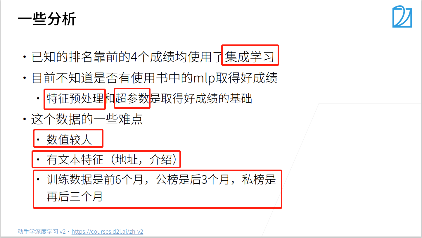
竞赛大佬方法:(它们都是使用集成学习的方法,来集成学习多个模型)
第二名和第七名:autogluon
第三名:h2o
第四名:随机森林
代码实现
导入相关库
import numpy as np
import pandas as pd
import torch
from torch import nn
from d2l import torch as d2l
1. 读取数据集
train_data = pd.read_csv('..\\data\\kaggle\\california-house-prices\\train.csv')
test_data = pd.read_csv('..\\data\\kaggle\\california-house-prices\\test.csv')
查看数据集的形状
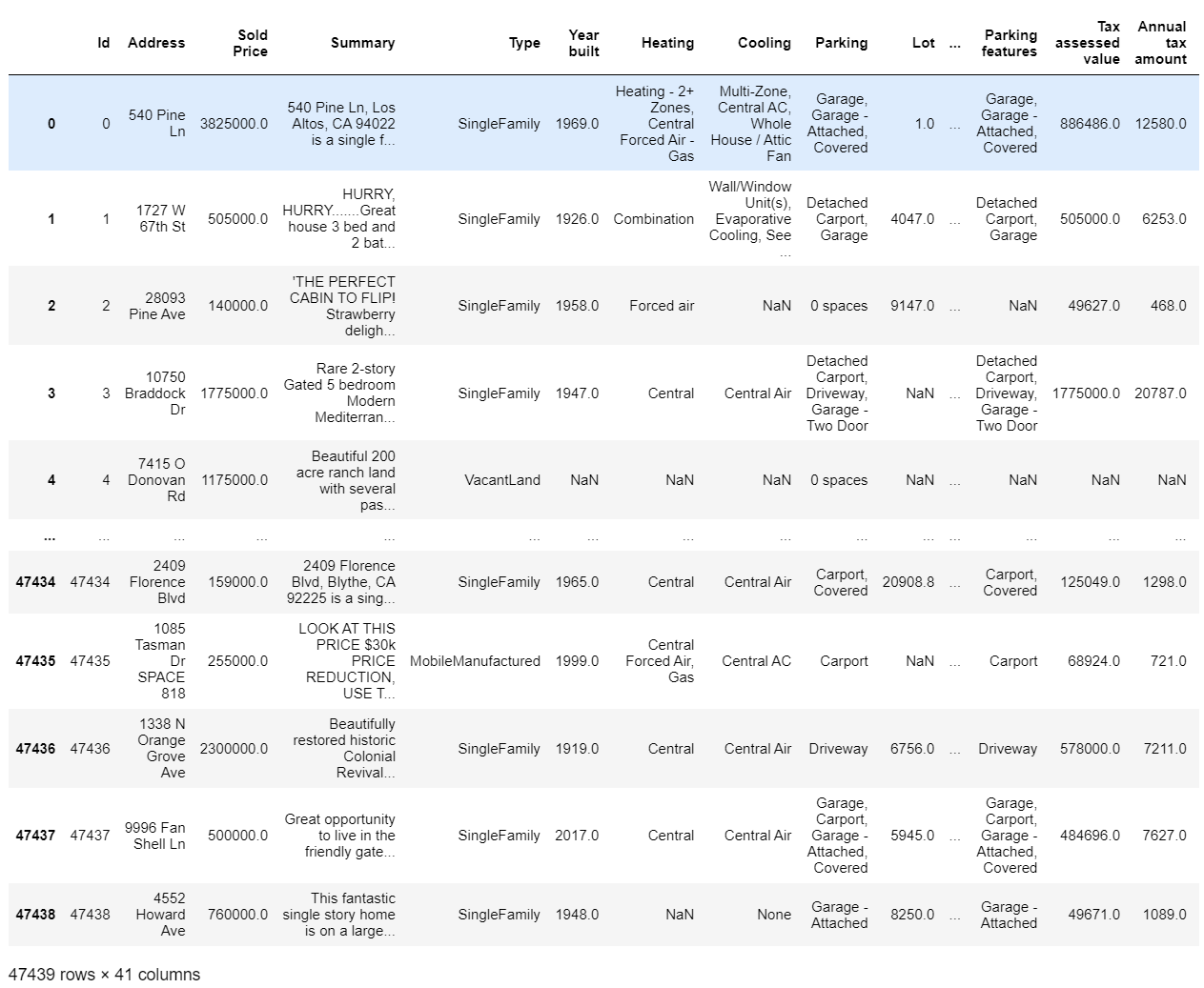
- 训练集的样本数为47439,列数为41(其中特征数为40,有1个为真实的房价(标签))
- 测试集的样本数为31626,列数为40(其中特征数为40, 没有标签)
print(train_data.shape, test_data.shape)

查看数据集train_data比test_data多一列:Sold Price(就是我们要预测的房价)
[i for i in train_data.columns if i not in test_data.columns]

看一下数据集的具体样子
train_data
2. 数据预处理
2.1 特征选择
- 因为41个特征中有一些特征是不需要的,如id、State…
- 由于Kaggle内存有限,需要选择一些较好的特征, 以免内存溢出
- 对于一些相对不好的特征,可能使最终训练的模型精度不高。
查看训练集和测试集的特征名称
# 查看特征
# train_data.columns,test_data.columns
其中部分特征:
- Type(房子类型:单体别墅、连体别墅)
- Year built(建筑时间,日期型数据)
- Heating(暖气),Cooling(空调),Parking(车库)
- Lot(占地面积多少)
- Bedrooms(卧室),Bathrooms(半洗手间:不能洗澡),Full bathrooms(洗手间:可以洗澡)
- Total interior livable area(居住面积),Total spaces(整体面积),Garage spaces(车库大小)
- Region(所在地区)
- Elementary School’, ‘Elementary School Score’,‘Elementary School Distance’, ‘Middle School’, ‘Middle School Score’,‘Middle School Distance’, ‘High School’, ‘High School Score’,'High School Distance(是不是学区房,每个学校的排名)
- Flooring(地板种类), Heating features(暖气种类), Cooling features(空调种类),Appliances included(有无电器),Laundry features(洗设施),Parking features(停车设施)
- Tax assessed value(纳税:政府对你的估值),Annual tax amount(年税额:每年要交的税),
- Listed On(挂牌时间), Listed Price(要价:卖家出售的价格),
- Last Sold On(上次的出售时间),Last Sold Price(卖价:上次最终卖的钱)
- City(城市),Zip(邮编)
剔除特别不好的特征
- 0:Id(序号,是每个样本的唯一标识)
- 1:Address(具体地址,每个样本的门牌号是唯一)
- 2:Sold Price(售价,是标签)(测试集独有)
- 3:Summary(文本数据,太长,分析有限)(也可能很重要,但是现在没法处理)
- -1:State(所有的样本都是来自CA(加州))
由于去除了标签,可以将训练集和测试集合并:方便后续处理
all_features = pd.concat((train_data.iloc[:, 4:-1], test_data.iloc[:, 3:-1]))
查看所有样本的形状
all_features.shape # 样本数:47439+31626= 79065 特征数:41-5=36 40-4=36

查看特征中有哪些数据类型
# 查看特征中有哪些数据类型
all_features.dtypes.unique()

3.2 处理时间数据
查看时间数据
all_features['Year built'], all_features['Listed On'], all_features['Last Sold On']
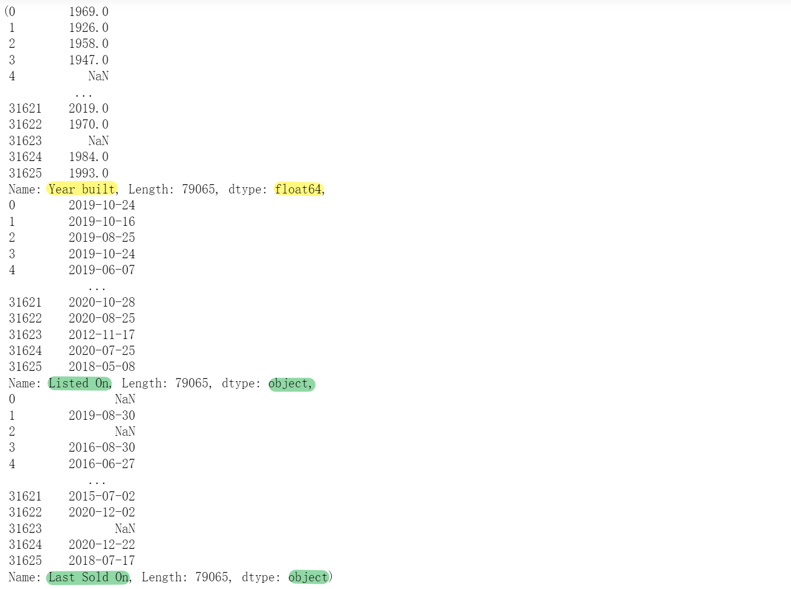
- Year built(dtype: float64):浮点型:不用处理
- Listed On(dtype: object)、Last Sold On(dtype: object):字符型,得转化为日期型
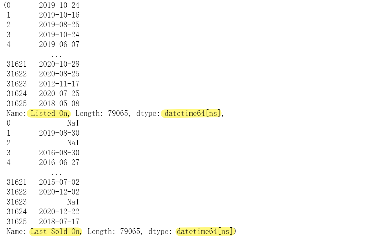
all_features['Listed On'] = pd.to_datetime(all_features['Listed On'], format="%Y-%m-%d")
all_features['Last Sold On'] = pd.to_datetime(all_features['Last Sold On'], format="%Y-%m-%d")
查看
all_features['Listed On'], all_features['Last Sold On']
2.3 处理数值型数据(17 +1(Year built) +2( Listed On、Last Sold On) = 20 )
- 首先,将所有数值型特征缩放到均值为0, 方差为1的正态分布,来标准化数据:(x - x.均值)/ x.标准差
- 然后,将所有缺失值替换为相应特征的平均值,即缺失值设置为0
numeric_features = all_features.dtypes[all_features.dtypes != 'object'].index
all_features[numeric_features] = all_features[numeric_features].apply(
    lambda x: (x - x.mean()) / (x.std()))
# 在标准化数据后,所有均值消失,因此我们可以将缺失值设置为0
all_features[numeric_features] = all_features[numeric_features].fillna(0)
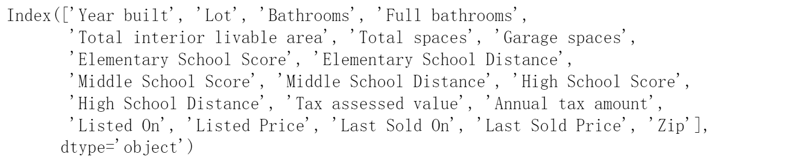
查看所有数值型特征的形状
all_features[numeric_features].shape

查看它们的特征名称是否与csv文件中的数值型特征一致
numeric_features
2.4 处理离散值型数据(1(Type))
用一次独热编码替换它们
- 如果对所有的离散值型数据都采用独热编码的格式来替换会发现,特征数高达49753,导致内存溢出
- 所以要对离散值型数据做进一步的筛选
查看所有的离散型数据
print(all_features.dtypes[all_features.dtypes =='object'])
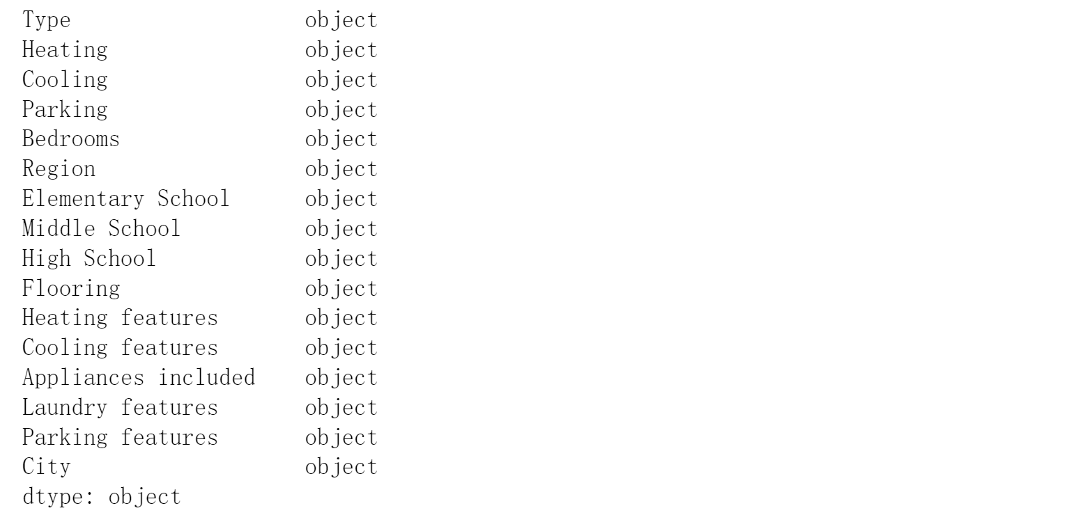
- 为了提高独热编码后,新特征的质量,我们看一下这些object类型中是否存在数据不一致的情况
object_numeric_features = all_features.dtypes[all_features.dtypes == 'object'].index
for i in object_numeric_features:
    print(len(all_features[i].unique()))
- 除了Type以外,其他数量很大的类别都是用逗号分隔的多类别文本数据。
- 因为现在水平有限,不太知道这种数据怎么编码,所以决定把它们都剔除掉
- 离散型数据特征仅使用Type
features = list(numeric_features)
features.append('Type')   # 加上类别数相对较少的Type
print(features)
现在新的特征数:21 (20: 数值型特征, 1:文本型特征)
all_features = all_features[features]  # 20 + 1 = 21
all_features.shape

- 将文本型特征进行独热编码
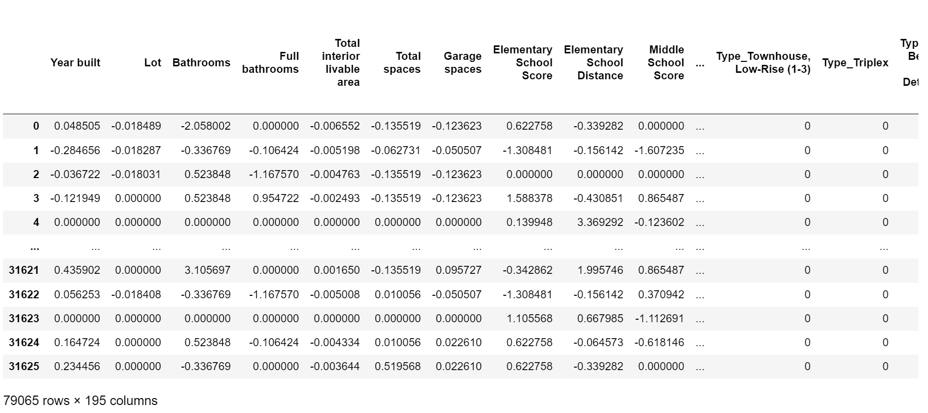
- 现在样本中的特征数为:21-1(Type)+174 + 1(na) = 195

查看样本
all_features
2.5 将特征的数据转换成tensor,并将其数据类型转换成float32
查看全部特征的数据类型
# 查看全部新特征的数据类型
all_features.dtypes.unique()

- 发现特征中任然有文本型
- 但是通过查看,发现文本型特征所在列和下标是空值,没有影响
- 特征中的数值型特征的数据类型有:’float64’, ‘uint8’,将其转换为float32。
print(all_features.dtypes[all_features.dtypes =='object'])

object_numeric_features = all_features.dtypes[all_features.dtypes == 'object'].index
object_numeric_features

n_train = train_data.shape[0]  # train_data.shape:[47439, 41]   train_data.shape[0]:47439
train_features = torch.tensor(all_features[:n_train].values, dtype=torch.float32)  # 训练集:前47439个样本
test_features = torch.tensor(all_features[n_train:].values, dtype=torch.float32)  # 验证集:后31626(79065-47439)个样本
train_labels = torch.tensor(train_data['Sold Price'].values.reshape(-1, 1), dtype=torch.float32)  # 训练集的标签
3. 定义训练函数
3.1. 是否使用GPU
# 是否使用GPU训练
if not torch.cuda.is_available():
    print('CUDA is not available.  Training on CPU ...')
else:
    print('CUDA is available.  Training on GPU ...')
device = torch.device("cuda:0" if torch.cuda.is_available() else "cpu")

3.2 定义网络模型
in_features = train_features.shape[1]

def get_net():
    net = nn.Sequential(
        nn.Linear(in_features, 1024), nn.ReLU(),  # in_features = 47439
        nn.Linear(1024, 512), nn.ReLU(),
        nn.Linear(512, 256), nn.ReLU(),
        nn.Linear(256, 128), nn.ReLU(),  # 5--折验证:平均训练log rmse:0.241757,平均验证log rmse: 0.277515
#         nn.Linear(128, 64), nn.ReLU(),  # 5--折验证:平均训练log rmse:0.268310,平均验证log rmse: 0.304618
        nn.Linear(128, 1))

    return net
3.3 定义损失函数
- 使用log_rmse(相对误差)来计算损失
- 因为不同房子的房价的差异较大,有时候1个房10w,另一个房100w,所以要用相对误差,而不是绝对误差。代码直接求的是log(y_hat/y),这样当y_hat越接近y,loss越小
loss = nn.MSELoss()


def log_rmse(net, features, labels):
    # 为了在取对数时进一步稳定该值, 将小于1的值设置为1
    clipped_preds = torch.clamp(net(features), 1, float('inf'))
    # torch.clamp()函数的功能将输入input张量每个元素的值压缩到区间 [1,+∞],并返回结果到一个新张量。
    rmse = torch.sqrt(loss(torch.log(clipped_preds), torch.log(labels)))  # rmse = log(y_hat)与log(y)的均方损误差在平方
    # torch.sqrt():逐元素计算张量的平方根
    return rmse.item()
3.4 定义训练函数
def train(net, train_features, train_labels, test_features, test_labels,
          num_epochs, learning_rate, weight_decay, batch_size):

    net = net.to(device)  # ---------------------模型传入GPU----------------

    train_ls, test_ls = [], []
    train_iter = d2l.load_array((train_features, train_labels), batch_size)
    optimizer = torch.optim.Adam(net.parameters(), lr=learning_rate, weight_decay=weight_decay)
    for epoch in range(num_epochs):
        for X, y in train_iter:
            X=X.to(device)  # ---------------------输入传入GPU----------------
            y=y.to(device)  # ---------------------标签传入GPU----------------
            optimizer.zero_grad()
            l = loss(net(X), y).to(device)  # ---------------------损失传入GPU----------------
            l.backward()
            optimizer.step()
        train_ls.append(log_rmse(net, train_features, train_labels))
        if test_labels is not None:
            test_ls.append(log_rmse(net, test_features, test_labels))
    return train_ls, test_ls
3.5 定义K则交叉验证函数
def get_k_fold_data(k, i, X, y):
    """把数据分为k块,将第i块拿出来作为验证集,其余k-1块重新合并作为训练集"""
    assert k > 1
    fold_size = X.shape[0] // k
    X_train, y_train = None, None
    for j in range(k):
        idx = slice(j * fold_size, (j + 1) * fold_size)  # 一折有多少个样本
        X_part, y_part = X[idx, :], y[idx]
        if j == i:  # i表示第几折:
            X_valid, y_valid = X_part, y_part  # j == i:将第i折作为验证集
        elif X_train is None:  # 表示第一次出现
            X_train, y_train = X_part, y_part  # 就把这一折存起来,作为训练集
        else:
            # torch.cat():将两个张量(tensor)按指定维度拼接在一起
            X_train = torch.cat([X_train, X_part], 0)    # 否则,就把X_train与其余折数据合并作为验证集
            y_train = torch.cat([y_train, y_part], 0)
    return X_train, y_train, X_valid, y_valid
3.6 带有K则交叉验证的训练函数
def k_fold(k, X_train, y_train, num_epochs, learning_rate, weight_decay, batch_size):
"""返回训练和验证误差的平均值"""
train_l_sum, valid_l_sum = 0, 0
for i in range(k):
data = get_k_fold_data(k, i, X_train, y_train)
net = get_net().to(device) # ---------------------模型传入GPU----------------
train_ls, valid_ls = train(net, *data, # *是解码,变成前面返回的四个数值
num_epochs, learning_rate, weight_decay, batch_size)
# [-1]:
# train函数返回的是整个训练中所有epoch的训练和验证损失数组,数组中每个元素是每一轮计算的损失
# 用-1表示(只取最后一轮的损失)最后一个epoch来代表这一折训练的效果
train_l_sum += train_ls[-1]
valid_l_sum += valid_ls[-1]
if i == 0: # 从0开始画图
d2l.plot(list(range(1, num_epochs + 1)), [train_ls, valid_ls],
xlabel='epoch', ylabel='rmse', xlim=[1, num_epochs],
legend=['train', 'valid'], yscale='log')
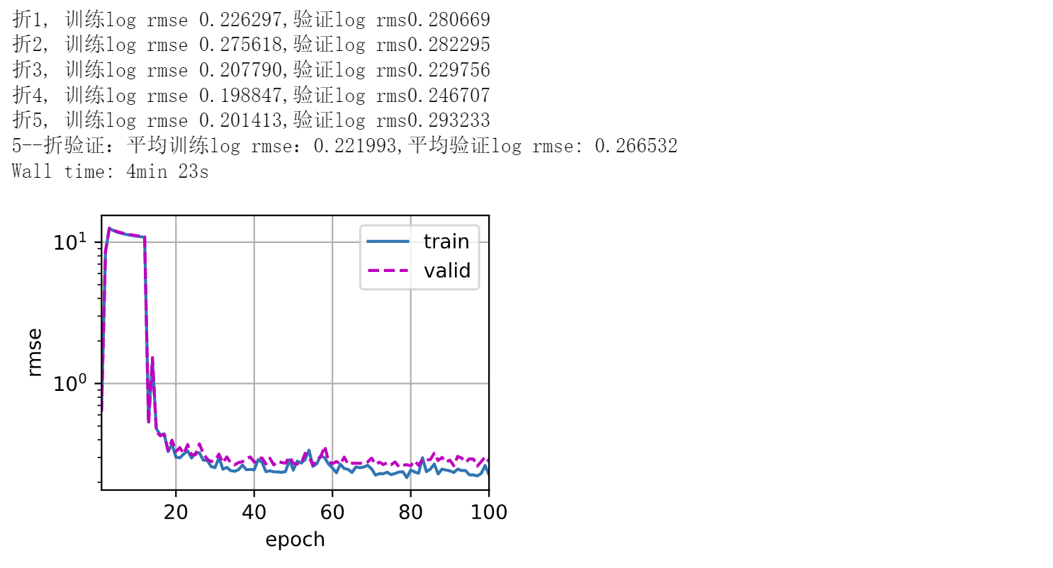
print(f'折{i + 1}, 训练log rmse {float(train_ls[-1]):f},'
f'验证log rms{float(valid_ls[-1]):f}')
return train_l_sum / k, valid_l_sum / k
4. 训练
%%time
train_features = train_features.to(device)  # ---------------------输入传入GPU----------------
train_labels = train_labels.to(device)  # ---------------------标签传入GPU----------------

k, num_epochs, lr, weight_decay, batch_size = 5, 100, 0.01, 0.01, 256
train_l, valid_l = k_fold(k, train_features, train_labels,
                          num_epochs, lr, weight_decay, batch_size)
print(f'{k}--折验证:平均训练log rmse:{float(train_l):f},'
      f'平均验证log rmse: {float(valid_l):f}')
5. 测试并保存
def train_and_pred(train_features, test_featrue, train_labels, test_data,
num_epochs, lr, weight_decay, batch_size):
net = get_net().to(device) # ---------------------模型传入GPU----------------
train_ls, _ = train(net, train_features, train_labels, None, None,
num_epochs, lr, weight_decay, batch_size)
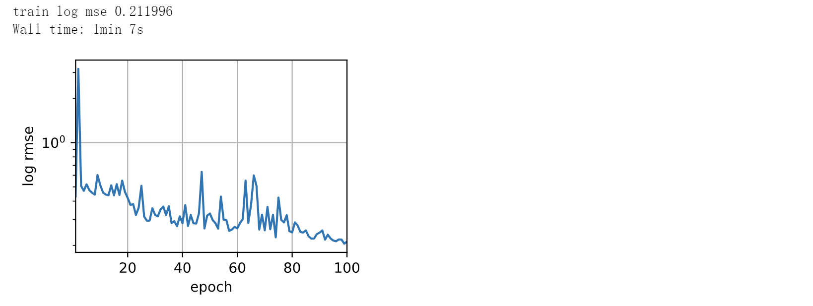
d2l.plot(np.arange(1, num_epochs + 1), [train_ls], xlabel='epoch',
ylabel='log rmse', xlim=[1, num_epochs], yscale='log')
print(f'train log mse {float(train_ls[-1]):f}')
# 将网络应用于测试集。
preds = net(test_featrue).detach().cpu().numpy()
# 将其重新格式化以导出到Kaggle
test_data['SalePrice'] = pd.Series(preds.reshape(1, -1)[0])
submission = pd.concat([test_data['Id'], test_data['SalePrice']], axis=1)
submission.to_csv('submission.csv', index=False)
%%time
test_features = test_features.to(device)  # ---------------------测试输入传入GPU----------------
train_features = train_features.to(device)  # ---------------------训练输入传入GPU----------------
train_labels = train_labels.to(device)  # ---------------------训练标签传入GPU----------------
train_and_pred(train_features, test_features, train_labels, test_data,
               num_epochs, lr, weight_decay, batch_size)