摘要
线性规划和逻辑回归分别是回归(regression) 和分类 (classification) 问题中最常见的算法之一。许多软件比如 Python, R 等都提供了相关的函数。这里我们介绍如何用 tensorflow 来进行简单的线性规划和逻辑回归。
Tensorflow 中单变量线性回归
假设我们的数据是
(
x
i
,
y
i
)
,
i
=
1
,
2
,
⋯
,
m
(x_i, \, y_i), \, i = 1, 2, \cdots, m
(xi,yi),i=1,2,⋯,m,即一共有
m
m
m 个数据点。我们须要根据
x
i
x_i
xi 来对
y
i
y_i
yi 进行预测。
在单变量的线性规划模型中,我们须要拟合
y
=
w
x
+
b
y = w x + b
y=wx+b。这里
y
y
y 就是要预测的值,
x
x
x 是我们的feature 值。我们想要用 tensorflow 来根据给出的数据
(
x
i
,
y
i
)
(x_i, \, y_i)
(xi,yi) 求解出
w
w
w 和
b
b
b 的值。根据最小二乘法的规定,为了求出
w
w
w 和
b
b
b,我们须要求出使得
RSS
=
∑
i
=
1
n
(
y
i
−
(
b
+
w
x
i
)
)
2
\displaystyle \text{RSS} = \sum_{i = 1}^n \left( y_i - (b + w x_i) \right)^2
RSS=i=1∑n(yi−(b+wxi))2
最小的
w
,
b
w, b
w,b。
在tensorflow中,我们通过定义损失函数(cost function),来求得使得 RSS (residual sum of squares) 最小的
w
,
b
w, b
w,b。具体代码如下。
import tensorflow.compat.v1 as tf
tf.disable_v2_behavior()
import numpy as np
import matplotlib.pyplot as plt
class demo_tensorflow:

    def __init__(self, X, Y):
        self.X = X
        self.Y = Y

    def tf_linear_regression(self, learning_rate, training_epoches):
        """
        Use tensorflow for linear regression.
        """
        # define X and Y. We will fit Y using X.
        X = tf.placeholder(tf.float32)
        Y = tf.placeholder(tf.float32)

        # w and b are the parameters that we need to fit
        w = tf.Variable(np.random.normal(), name="weights")
        b = tf.Variable(np.random.normal(), name='intercept')

        # define the model
        model = tf.add(tf.multiply(X, w), b)

        # define the cost function
        cost = tf.reduce_mean(tf.square(model - Y))

        train_op = tf.train.GradientDescentOptimizer(learning_rate).minimize(cost)

        with tf.Session() as sess:
            sess.run(tf.global_variables_initializer())
            for epoch in range(training_epoches):
                sess.run(train_op, feed_dict={X: self.X, Y: self.Y})
                cur_cost = sess.run(cost, feed_dict={X: self.X, Y: self.Y})
                if (epoch + 1) % 500 == 1:
                    print("Epoch", (epoch + 1), ": cost=", cur_cost)
            weight = sess.run(w)
            intecept = sess.run(b)
        return weight, intecept
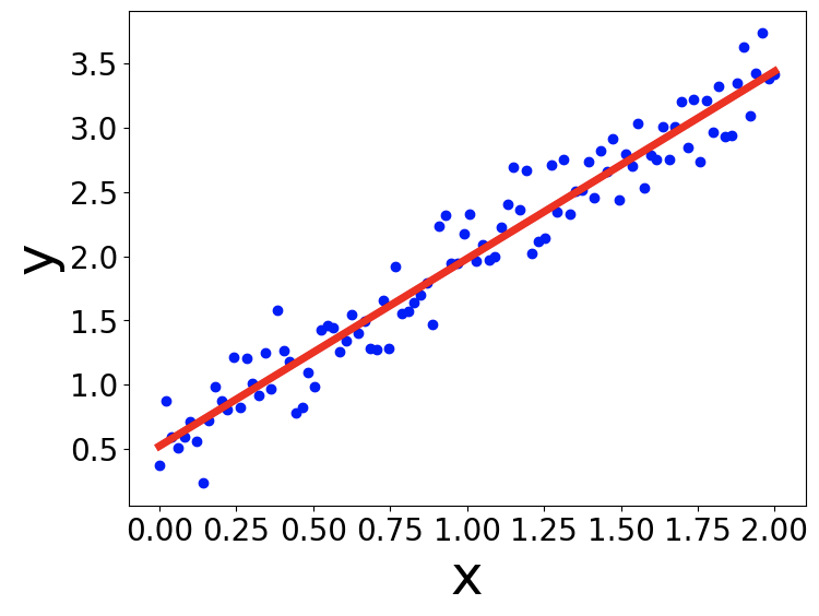
x_batch = np.linspace(0, 2, 100) # training x data
y_batch = 1.5 * x_batch + np.random.randn(*x_batch.shape) * 0.2 + 0.5 # training y data
learning_rate = 0.01
training_epoches = 5000
a = demo_tensorflow(x_batch, y_batch)
a.tf_linear_regression(learning_rate, training_epoches)
Epoch 1 : cost= 2.3156583
Epoch 501 : cost= 0.045759827
Epoch 1001 : cost= 0.045451876
Epoch 1501 : cost= 0.04543826
Epoch 2001 : cost= 0.04543766
Epoch 2501 : cost= 0.04543763
Epoch 3001 : cost= 0.045437638
Epoch 3501 : cost= 0.045437627
Epoch 4001 : cost= 0.045437627
Epoch 4501 : cost= 0.045437627
根据训练模型得到的直线如下图所示。
多变量的情况
对于多变量的情况,我们只须要在定义 tf.placeholder 和 tf.Variable 的时候注意矩阵的维度。其余部分是相同的。值得注意的是,我们应该用tf.matmul 来对矩阵进行乘法运算。具体代码如下 [1]。
def tf_multi_linear_regression(self, learning_rate, training_epoches):
        """
        multivariate case for linear regression.
        """
        # m is the number of training data, p is the number of features
        m, p = self.X.shape
        #print(m, p)
        # define X and Y. We will fit Y using X.
        X = tf.placeholder(tf.float32, shape=(None, p))
        Y = tf.placeholder(tf.float32, shape=(None, 1))

        # w and b are the parameters that we need to fit
        w = tf.Variable(tf.random_normal([p, 1], stddev=0.01), dtype=np.float32, name="weights")
        b = tf.Variable(np.random.normal(), dtype=np.float32, name='intercept')
        # define the model
        model = tf.add(tf.matmul(X, w), b) # Note that we use tf.matmul for matrix multicplication.

        # define the cost function
        cost = tf.reduce_mean(tf.square(model - Y))

        train_op = tf.train.GradientDescentOptimizer(learning_rate).minimize(cost)

        with tf.Session() as sess:
            sess.run(tf.global_variables_initializer())
            for epoch in range(training_epoches):
                sess.run(train_op, feed_dict={X: np.asarray(self.X), Y: np.asarray(self.Y).reshape(m, 1)})
                cur_cost = sess.run(cost, feed_dict={X: np.asarray(self.X), Y: np.asarray(self.Y).reshape(m, 1)})
                if (epoch + 1) % 500 == 1:
                    print("Epoch", (epoch + 1), ": cost=", cur_cost)
            weight = sess.run(w)
            intecept = sess.run(b)
        return weight, intecept
m = 10 ** 2
x1 = np.linspace(0, 2, m)
x2 = np.linspace(-1, 2, m) + np.random.normal(0, 2, m)
x_multi = np.vstack((x1, x2)).T
y = -2 * x1 + 3 * x2 + 2 + np.random.normal(0, 1, m) * 0.2
a = demo_tensorflow(x_multi, y)
a.tf_multi_linear_regression(learning_rate, training_epoches)
Epoch 1 : cost= 36.237904
Epoch 501 : cost= 0.1619576
Epoch 1001 : cost= 0.03932593
Epoch 1501 : cost= 0.033134725
Epoch 2001 : cost= 0.03282215
Epoch 2501 : cost= 0.032806374
Epoch 3001 : cost= 0.032805584
Epoch 3501 : cost= 0.032805543
Epoch 4001 : cost= 0.032805547
Epoch 4501 : cost= 0.032805547
(array([[-2.016268 ],
[ 3.0005507]], dtype=float32), 2.020361)
用 tensorflow进行逻辑回归分类
有了用tensorflow 进行线性回归的经验之后,对于用罗辑回归(logistic regression) 进行分类,我们只需要定义新的损失函数,而其他大部分代码与线性回归的情况。对于数据
(
x
i
,
y
i
)
,
i
=
1
,
2
,
⋯
,
m
(x_i, \, y_i), \, i = 1, 2, \cdots, m
(xi,yi),i=1,2,⋯,m,
y
i
∈
{
0
,
1
}
y_i \in \{0, \, 1\}
yi∈{0,1}。逻辑回归的损失函数定义为:
cost
=
−
1
m
∑
i
=
1
m
(
y
i
log
(
y
i
^
)
+
(
1
−
y
i
)
log
(
1
−
y
i
^
)
)
\text{cost} = -\frac{1}{m} \sum_{i = 1}^m \left( y_i \log(\hat{y_i}) + (1 - y_i) \log(1 - \hat{y_i}) \right)
cost=−m1i=1∑m(yilog(yi^)+(1−yi)log(1−yi^))
这里
y
i
^
\displaystyle \hat{y_i}
yi^ 是我们预测数据
x
i
x_i
xi 属于类别 1 的概率。具体的表达式为:
y
i
^
=
σ
(
w
x
i
+
b
)
\hat{y_i} = \sigma(w x_i + b)
yi^=σ(wxi+b)。
其中
σ
\sigma
σ 函数是 sigmoid 函数,
σ
(
x
)
=
1
1
+
e
−
x
\sigma(x) = \frac{1}{1 + e^{-x}}
σ(x)=1+e−x1。可以看出
0
<
σ
(
x
)
<
1
,
∀
x
∈
R
0 < \sigma(x) < 1, \forall x \in \mathbb{R}
0<σ(x)<1,∀x∈R,所以
y
i
^
\hat{y_i}
yi^ 作为概率始终是有意义的。
有了 cost 函数,我们便可以用 tensorflow 中的 optimization 方法进行优化,求出参数
w
w
w 和
b
b
b。具体代码如下:
class demo_tf_logisticRegression:

    def __init__(self, X, Y):
        self.X = X
        self.Y = Y


    def tf_logistic_regression(self, learning_rate, training_epoches):
        """
        Train the logistic regression model using tensorflow.
        """
        # m is the number of training data points, p is the number of features.
        m, p = self.X.shape
        X = tf.placeholder(tf.float32, shape=(None, p))
        Y = tf.placeholder(tf.float32, shape=(None, 1))

        w = tf.Variable(tf.random_normal([p, 1]), dtype=tf.float32, name='weights')
        b = tf.Variable(np.random.normal(), dtype=tf.float32, name='bias')

        model = tf.sigmoid(tf.add(tf.matmul(X, w), b))
        cost = -tf.reduce_mean(Y * tf.log(model) + (1 - Y) * tf.log(1 - model))

        train_op = tf.train.GradientDescentOptimizer(learning_rate).minimize(cost)

        with tf.Session() as sess:
            sess.run(tf.global_variables_initializer())
            for epoch in range(training_epoches):
                sess.run(train_op, feed_dict={X: np.asarray(self.X), Y: np.asarray(self.Y).reshape(m, 1)})
                cur_cost = sess.run(cost, feed_dict={X: np.asarray(self.X), Y: np.asarray(self.Y).reshape(m, 1)})
                if (epoch + 1) % 500 == 1:
                    print("Epoch", (epoch + 1), ": cost=", cur_cost)
            weight = sess.run(w)
            intecept = sess.run(b)
        return weight, intecept

    def get_boundary(self, w, b):
        """
        Obtain the classification boundary using the weight and bias that we got from the
        training.
        """
        x_boundary, y_boundary = [], []
        for x in np.linspace(0, 3, 100):
            for y in np.linspace(-1, 5, 100):
                prob = self.sigmoid(w[0] * x + w[1] * y + b)
                if np.abs(prob - 0.5) < 0.01:
                    x_boundary.append(x)
                    y_boundary.append(y)
        return x_boundary, y_boundary

    def sigmoid(self, x):
        """
        define the sigmoid function
        """
        return 1 / (1 + np.exp(-x))
假如我们要对下图中的红点(标记为0)和蓝点(标记为1)进行分类。那么我们用逻辑回归得到的分类边界如下图中绿线所示。
# Define the training data
np.random.seed(2)
m = 100
x1 = np.random.uniform(0, 3, m)
y1 = x1 - 1 + np.random.normal(0, 1, m) # with label 0
x2 = np.random.uniform(0, 3, m)
y2 = x2 + 1 + np.random.normal(0, 1, m) # with label 1
x_train_0 = np.vstack((x1, y1))
x_train_1 = np.vstack((x2, y2))
x_train = np.hstack((x_train_0, x_train_1)).T
y_train = np.asarray([0] * m + [1] * m)
# train the logistic model with tensorflow
b = demo_tf_logisticRegression(x_train, y_train)
w, bias = b.tf_logistic_regression(learning_rate, training_epoches)
x_b, y_b = b.get_boundary(w, bias)
Epoch 1 : cost= 1.7830517
Epoch 501 : cost= 0.5220195
Epoch 1001 : cost= 0.44926476
Epoch 1501 : cost= 0.4294767
Epoch 2001 : cost= 0.4218148
Epoch 2501 : cost= 0.41830078
Epoch 3001 : cost= 0.41651848
Epoch 3501 : cost= 0.41554946
Epoch 4001 : cost= 0.41499367
Epoch 4501 : cost= 0.41466048
# plot the data points and the classification boundary
# learned from tensorflow
plt.figure(figsize=(8, 6), dpi=100)
plt.plot(x1, y1, 'o', color='red', markersize=10)
plt.plot(x2, y2, 's', color='blue', markersize=10)
plt.plot(x_b, y_b, '-', color='green', linewidth = 5)
plt.xlabel('x', fontsize = 20)
plt.ylabel('y', fontsize = 20)
plt.xticks(fontsize=20)
plt.yticks(fontsize=20)

参考文献
[1] Machine learning with tensorflow, Nishant Shukla, Manning Publications, 2017