k-近邻算法是一种常用的监督学习算法,用于分类和回归任务。其思想为:如果一个样本在特征空间中的k个最近邻居中的大多数属于某个类别,那么该样本也属于这个类别(对于分类任务)或者可以通过这些最近邻居的标签来估计其目标值(对于回归任务)。
def createDataSet ( ) :
'''
构造数据
Parameters:
None
Returns:
group - 数据
labels - 标签
'''
group = array( [ [ 100 , 98 ] , [ 100 , 100 ] , [ 0 , 0 ] , [ 0 , 10 ] ] ) #[测试1的得分,测试2的得分]
labels = [ 'A' , 'A' , 'B' , 'B' ] #整体评级情况
return group, labels
通过计算两点之间的距离来进一步选择相近的k个点:
d
=
(
x
A
0
−
x
B
0
)
2
−
(
x
A
1
−
x
B
1
)
2
d=\sqrt{(x_{A_0}-x_{B_0})^2-(x_{A_1}-x_{B_1})^2}
d = ( x A 0 − x B 0 ) 2 − ( x A 1 − x B 1 ) 2
def classify_KNN ( inX, dataSet, labels, k) :
'''
使用kNN算法进行分类
Parameters:
inX - 用于分类的数据(测试集)
dataSet - 用于训练的数据(训练集)
labels - 训练集标签
k - kNN算法参数,选择距离最小的k个点
Returns:
sortedClassCount - 分类结果
'''
dataSetSize = dataSet. shape[ 0 ] #dataSet的行数
diffMat = inX - dataSet #计算差值矩阵-广播
sqDiffMat = diffMat** 2 #差值矩阵平方
sqDistances = sqDiffMat. sum ( axis= 1 ) #计算平方和
distances = sqDistances** 0.5 #开根号
sortedDistIndicies = distances. argsort( ) #获取升序索引
classCount= { }
for i in range ( k) :
voteIlabel = labels[ sortedDistIndicies[ i] ] #获得类别信息
classCount[ voteIlabel] = classCount. get( voteIlabel, 0 ) + 1 #类别数量+1
sortedClassCount = sorted ( classCount. items( ) , key= operator. itemgetter( 1 ) , reverse= True )
return sortedClassCount[ 0 ] [ 0 ]
至此,就可以通过给定数据进行分类预测,分类预测的效果与数据集的标准
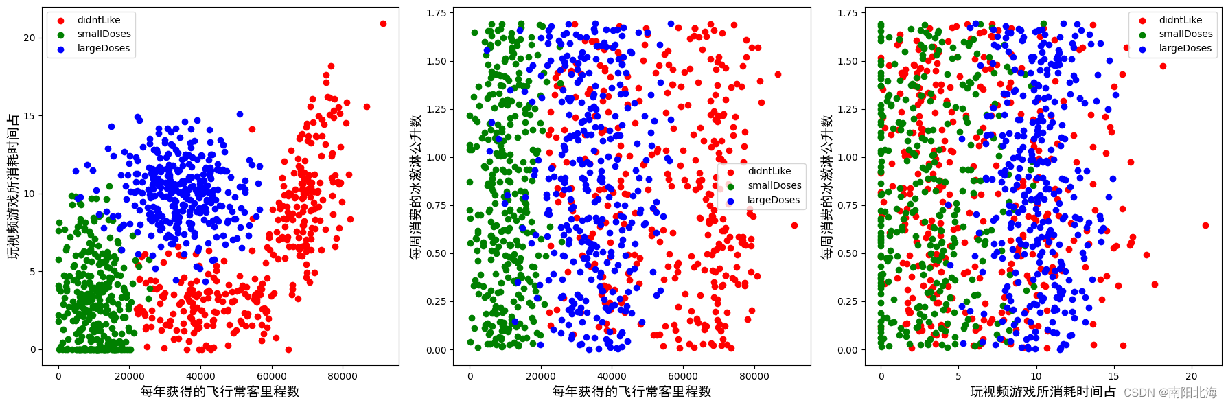
海伦将自己交往过的人可以进行如下分类:不喜欢的人、魅力一般的人、极具魅力的人。
def file2matrix ( filename) :
'''
读取数据,并将其转化为矩阵
Parameters:
filename - 文件路径
Returns:
returnMat - 数据矩阵
classLabelVector - 数据标签
'''
with open ( filename, "r" ) as file :
lines = file . readlines( ) #读取文本信息
numberOfLines = len ( lines) #计算行数
returnMat = zeros( ( numberOfLines, 3 ) ) #初始化矩阵
classLabelVector = [ ] #创建分类标签向量
index = 0
for line in lines:
line = line. strip( )
listFromLine = line. split( '\t' )
returnMat[ index, : ] = listFromLine[ 0 : 3 ]
#根据文本中标记的喜欢的程度进行分类,1代表不喜欢,2代表魅力一般,3代表极具魅力
if listFromLine[ - 1 ] == 'didntLike' :
classLabelVector. append( 1 )
elif listFromLine[ - 1 ] == 'smallDoses' :
classLabelVector. append( 2 )
elif listFromLine[ - 1 ] == 'largeDoses' :
classLabelVector. append( 3 )
index += 1
return returnMat, classLabelVector #(1000, 3),(1000,)
对于不同的类别的数据分布差异可能比较大,例如游戏时长百分比的差异在0-1之间,而飞行里程往往差异成败上千不等,差异大的属性值会严重影响欧式距离。因此需要对数据进行标准化,计算公式如下:
d
a
t
a
n
o
r
m
=
d
a
t
a
−
d
a
t
a
m
i
n
d
a
t
a
m
a
x
−
d
a
t
a
m
i
n
data_{norm} = \frac{data-data_{min}}{data_{max}-data_{min}}
d a t a n or m = d a t a ma x − d a t a min d a t a − d a t a min
def autoNorm ( dataSet) :
'''
归一化dataset中的值,函数返回归一化后的数据
Parameters:
dataSet - 原始数据
Returns:
normDataSet - 归一化后的数据
ranges - 最大最小值的差值
minVals - 数据中的最小值
'''
minVals = dataSet. min ( 0 ) #获得数据的最小值
maxVals = dataSet. max ( 0 ) #获得数据的最大值
ranges = maxVals - minVals#最大值和最小值的范围
normDataSet = zeros( shape( dataSet) ) #初始化归一矩阵
m = dataSet. shape[ 0 ] #dataSet的行数
normDataSet = dataSet - tile( minVals, ( m, 1 ) ) #原始值减去最小值,tile是扩充函数
normDataSet = normDataSet / tile( ranges, ( m, 1 ) ) #除以最大和最小值的差,得到归一化数据
return normDataSet, ranges, minVals
def showdatas ( datingDataMat, datingLabels) :
'''
将数据以散点图形式展示出来。
Parameters:
datingDataMat - 数据矩阵
datingLabels - 数据标签
Returns:
None
'''
color_map = { 1 : 'r' , 2 : 'g' , 3 : 'b' } # 创建颜色映射,将每个标签映射到不同的颜色
label_name = [ 'didntLike' , 'smallDoses' , 'largeDoses' ]
# 根据标签分组数据点
grouped_data = { }
for label in np. unique( datingLabels) :
grouped_data[ label] = datingDataMat[ datingLabels == label]
plt. figure( figsize= ( 18 , 6 ) )
plt. subplot( 131 ) # 创建X-Y平面上的散点图
for label, color in color_map. items( ) :
points = grouped_data[ label]
plt. scatter( points[ : , 0 ] , points[ : , 1 ] , c= color, label= f' { label_name[ label- 1 ] } ' )
plt. xlabel( '每年获得的飞行常客里程数' , fontproperties= font)
plt. ylabel( '玩视频游戏所消耗时间占' , fontproperties= font)
plt. legend( )
# 创建X-Z平面上的散点图
plt. subplot( 132 )
for label, color in color_map. items( ) :
points = grouped_data[ label]
plt. scatter( points[ : , 0 ] , points[ : , 2 ] , c= color, label= f' { label_name[ label- 1 ] } ' )
plt. xlabel( '每年获得的飞行常客里程数' , fontproperties= font)
plt. ylabel( '每周消费的冰激淋公升数' , fontproperties= font)
plt. legend( )
# 创建Y-Z平面上的散点图
plt. subplot( 133 )
for label, color in color_map. items( ) :
points = grouped_data[ label]
plt. scatter( points[ : , 1 ] , points[ : , 2 ] , c= color, label= f' { label_name[ label- 1 ] } ' )
plt. xlabel( '玩视频游戏所消耗时间占' , fontproperties= font)
plt. ylabel( '每周消费的冰激淋公升数' , fontproperties= font)
plt. legend( )
# 显示图形
plt. tight_layout( )
plt. show( )
将数据按照指定比例划分训练集与测试集,训练集用于构建模型,测试集用于评估算法与数据的可靠性。
def datingClassTest ( ) :
"""
测试算法的准确度,打印出算法的错误率
Parameters:
None
Returns:
None
"""
filename = r"./datingTestSet.txt" #文件路径
datingDataMat, datingLabels = file2matrix( filename)
hoRatio = 0.10 #测试集比例
normMat, ranges, minVals = autoNorm( datingDataMat) #数据归一化
m = normMat. shape[ 0 ] #数据量
numTestVecs = int ( m * hoRatio) #测试集个数
errorCount = 0.0 #分类错误量
for i in range ( numTestVecs) : #遍历测试集,评估正确率
classifierResult = classify_KNN( normMat[ i, : ] , normMat[ numTestVecs: m, : ] , datingLabels[ numTestVecs: m] , 4 )
#输出错误的情况
if classifierResult != datingLabels[ i] :
errorCount += 1.0
print ( "分类结果:%d\t真实类别:%d" % ( classifierResult, datingLabels[ i] ) )
print ( "错误率:%f%%" % ( errorCount/ float ( numTestVecs) * 100 ) )
调用模型就可以进行数据的预估,不同的k值也可能会有不同的结果。需要根据实际应用场景决定
def classifyPerson ( ) :
"""
根据输入内容进行判断
Parameters:
None
Returns:
None
"""
resultList = [ '讨厌' , '有些喜欢' , '非常喜欢' ] #输出结果
precentTats = float ( input ( "玩视频游戏所耗时间百分比:" ) )
ffMiles = float ( input ( "每年获得的飞行常客里程数:" ) )
iceCream = float ( input ( "每周消费的冰激淋公升数:" ) )
filename = "./datingTestSet.txt"
datingDataMat, datingLabels = file2matrix( filename)
normMat, ranges, minVals = autoNorm( datingDataMat)
inArr = array( [ precentTats, ffMiles, iceCream] )
norminArr = ( inArr - minVals) / ranges
#返回分类结果
classifierResult = classify_KNN( norminArr, normMat, datingLabels, 3 )
#打印结果
print ( "你可能%s这个人" % ( resultList[ classifierResult- 1 ] ) )
对于手写识别系统而言整体流程是一致的,主要差距在于数据的输入以及预处理上。
def img2vector ( file_path) :
"""
将32x32的二进制图像转换为1x1024向量。
Parameters:
file_path - 文件名
Returns:
returnVect - 返回的二进制图像的1x1024向量
"""
returnVect = np. zeros( ( 1 , 1024 ) ) #初始化
with open ( file_path, 'r' ) as file :
for i in range ( 32 ) :
lineStr = file . readline( )
for j in range ( 32 ) :
returnVect[ 0 , 32 * i+ j] = int ( lineStr[ j] )
return returnVect