from scipy.io import loadmat
import numpy as np
import matplotlib.pyplot as plt
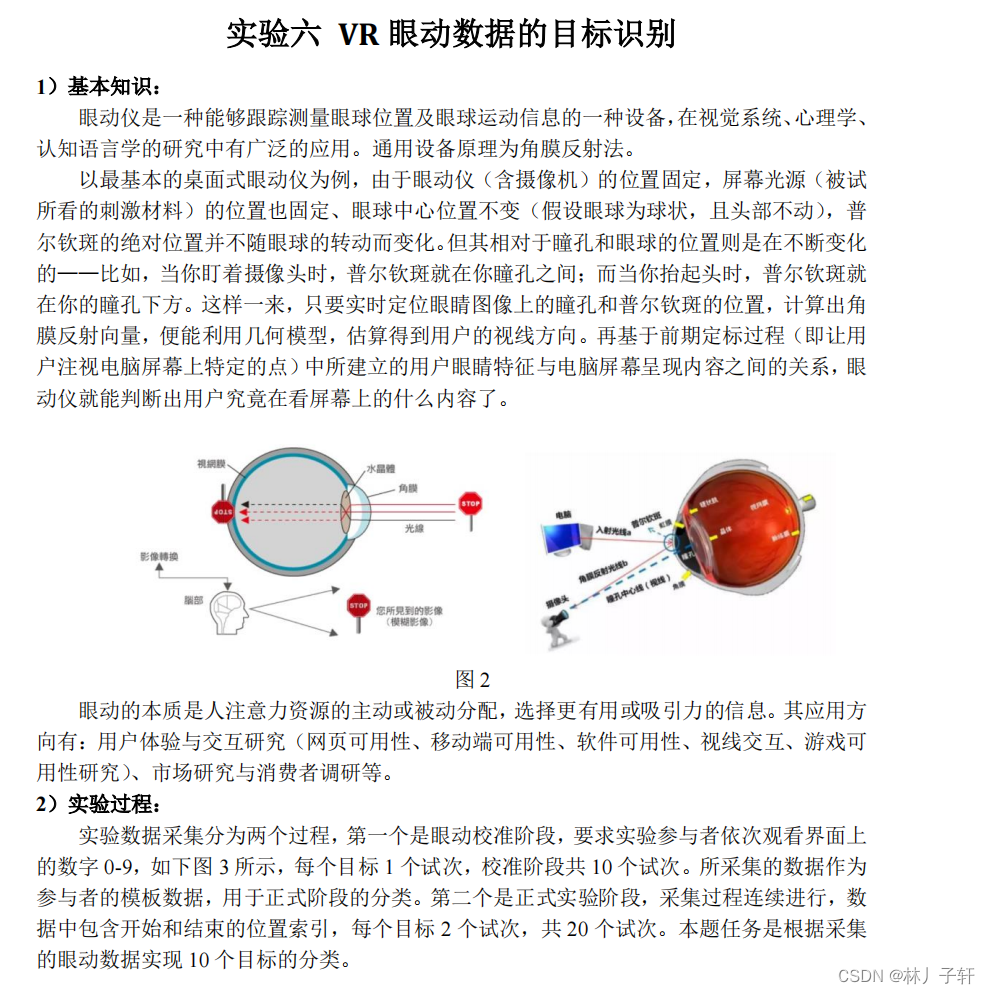
实验数据采集分为两个过程,
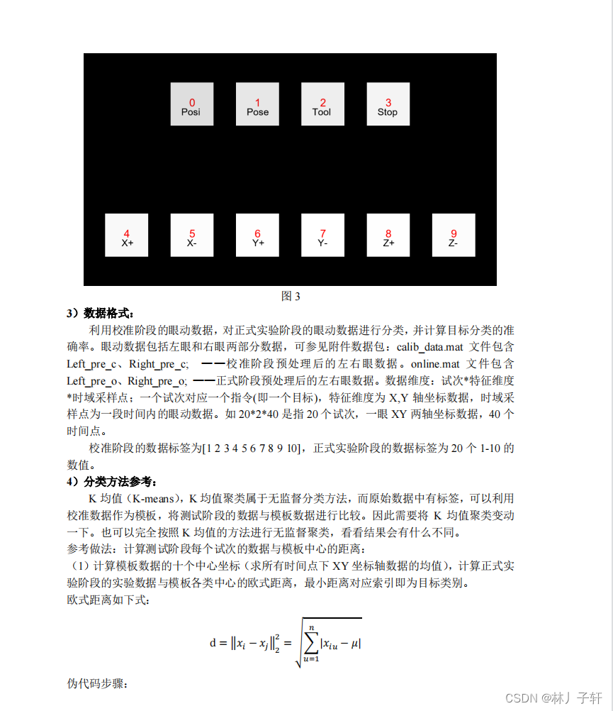
第一个是眼动校准阶段,要求实验参与者依次观看界面上的数字 0-9,
如下图 3 所示,每个目标 1 个试次,校准阶段共 10 个试次.
所采集的数据作为参与者的模板数据,用于正式阶段的分类.
第二个是正式实验阶段,采集过程连续进行,数据中包含开始和结束的位置索引,每个目标 2 个试次,共 20 个试次.
本题任务是根据采集的眼动数据实现 10 个目标的分类
dict_calib = loadmat("本科课设数据及说明-2021/sub-data/eyedata/calib_data.mat") #校准阶段数据,也就是数据模板
print(dict_calib.keys())
dict_label = loadmat("本科课设数据及说明-2021/sub-data/eyedata/label.mat")
print(dict_label.keys())
dict_online = loadmat("本科课设数据及说明-2021/sub-data/eyedata/online.mat")
print(dict_online.keys())
dict_keys(['__header__', '__version__', '__globals__', 'Left_pre_c', 'Right_pre_c'])
dict_keys(['__header__', '__version__', '__globals__', 'label'])
dict_keys(['__header__', '__version__', '__globals__', 'Left_pre_o', 'Right_pre_o'])
利用校准阶段的眼动数据,对正式实验阶段的眼动数据进行分类,
并计算目标分类的准确率。眼动数据包括左眼和右眼两部分数据,可参见附件数据包:
calib_data.mat 文件包含
Left_pre_c、Right_pre_c; ——校准阶段预处理后的左右眼数据.
online.mat 文件包含
Left_pre_o、Right_pre_o; ——正式阶段预处理后的左右眼数据。
数据维度:试次特征维度
校准阶段的数据标签为[1 2 3 4 5 6 7 8 9 10],正式实验阶段的数据标签为 20 个 1-10 的
数值.
时域采样点
一个试次对应一个指令(即一个目标),特征维度为 X,Y 轴坐标数据,
时域采样点
为一段时间内的眼动数据。如 20,2,40 是指 20 个试次,一眼 XY 两轴坐标数据,40 个时间点.
label = dict_label['label']
label = np.concatenate((label[:,0],label[:, 1]))
label
array([ 1,  2,  3,  4,  5,  6,  7,  8,  9, 10, 10,  9,  8,  7,  6,  5,  4,
        3,  2,  1], dtype=uint8)
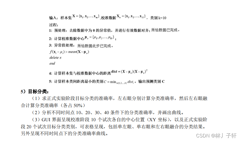
- 计算模板数据的十个中心坐标(求所有时间点下 XY 坐标轴数据的均值)
calib_data = dict_calib['Left_pre_c']  # (10, 2, 40)
module_coordinate = np.array([(label[0].mean(),label[1].mean()) for label in calib_data])
- 计算正式实验阶段的实验数据与模板各类中心的欧式距离,最小距离对应索引即为目标类别
def eucldist_vectorized(modules, coord):
    """
    :param modules: 模板数据  (n,2)
    :param coord: (2)
    :return: 最小值的下标
    """
    """ Calculates the euclidean distance between 2 lists of coordinates. """
    distant = []
    for module in modules:
        distant.append( np.sqrt(np.sum((module - coord)**2)))
    distant = np.array(distant)
    label = distant.argmin()
    return label+1

Left_o, Right_o = dict_online['Left_pre_o'], dict_online['Right_pre_o']  # (20, 2, 40), (20, 2, 40)

Left_o_mean = [[label[0].mean(),label[1].mean()] for label  in Left_o] # 20,2
Right_o_mean = [[label[0].mean(),label[1].mean()] for label  in Right_o] # 20,2

def get_mix_mean(left, right):
    Mix_o_mean = []
    for value in zip(left,right):
        x_mean = np.array([value[0][0],value[1][0]]).mean()
        y_mean = np.array([value[0][1],value[1][1]]).mean()
        Mix_o_mean.append([x_mean,y_mean])

    return np.array(Mix_o_mean)
Mix_o_mean = get_mix_mean(Left_o_mean, Right_o_mean)
print(Mix_o_mean.shape)
(20, 2)
(1)求正式实验阶段目标分类的准确率,左右眼分别计算分类准确率,然后左右眼融
合计算分类准确率(各占 50%)
(2)分析不同时间点 10、20、30、40 条件下的分类准确率,并画出曲线。
(3)GUI 界面呈现校准阶段 10 个试次各自的中心位置(XY 坐标),以及正式实验阶
段 20 个试次目标分类类别,可表格呈现,包括单左眼、单右眼和左右眼融合的分类结果。
另外呈现不同时间点下的分类准确率曲线.
# 求正式实验阶段目标分类的准确率,左右眼分别计算分类准确率,然后左右眼融合计算分类准确率(各占 50%)
def calculate_acc(preds, labels):
    """

    :param preds: 预测
    :param labels: 实际
    :return: acc
    """
    assert len(preds) == len(labels)
    count = 0
    for pred, label in zip(preds,labels):
        if pred == label:
            count +=1
    acc = count / len(preds)
    return acc

pred_left = [eucldist_vectorized(module_coordinate,coord) for coord in Left_o_mean]
pred_right = [eucldist_vectorized(module_coordinate,coord) for coord in Right_o_mean]
pred_mix = [eucldist_vectorized(module_coordinate,coord) for coord in Mix_o_mean]


print(f"pred_left acc is :{calculate_acc(pred_left, label)}")
print(f"pred_right acc is :{calculate_acc(pred_right, label)}")
print(f"pred_mix acc is :{calculate_acc(pred_mix, label)}")
pred_left acc is :0.95
pred_right acc is :0.45
pred_mix acc is :0.7
(2)分析不同时间点 10、20、30、40 条件下的分类准确率,并画出曲线.
此题中不同时间点, 理解为瞬间的准确率?
此处曲线, 横坐标4个点,中坐标 acc
# 40个采样点中取  4个时间点
time = [9, 19, 29, 39] # 数组从0开始,减1
sample = []
for t in time:
    left = Left_o[:,:,t]
    right = Right_o[:,:,t]
    mix = get_mix_mean(left,right)
    sample.append([left, right, mix])
sample = np.array(sample)
print(sample.shape)  # (4, 3, 20, 2)  4 个时间点, 3中类型,20个样本,2是数据维度(坐标)

plot_data = []
# # 计算分类准确率,画出曲线
for temp in sample:
    pred_left_sample = [eucldist_vectorized(module_coordinate,coord) for coord in temp[0]]
    pred_right_sample = [eucldist_vectorized(module_coordinate,coord) for coord in temp[1]]
    pred_mix_sample = [eucldist_vectorized(module_coordinate,coord) for coord in temp[2]]
    left_acc = calculate_acc(pred_left_sample, label)
    right_acc = calculate_acc(pred_right_sample, label)
    mix_acc = calculate_acc(pred_mix_sample, label)
    plot_data.append([left_acc, right_acc, mix_acc])


plt.rcParams['font.family'] = 'SimHei'
plot_data = np.array(plot_data)
plt.plot(plot_data[:,0], color = 'yellow', label='Left acc' )
plt.plot(plot_data[:,1], color = 'blue', label='Right acc' )
plt.plot(plot_data[:,2], color = 'red', label='Mix acc' )
plt.legend(loc='upper right')
plt.xlabel("4个采样点")
plt.ylabel(" Accuracy")
plt.show()
(4, 3, 20, 2)

(3)GUI 界面呈现校准阶段 10 个试次各自的中心位置(XY 坐标),以及正式实验阶
段 20 个试次目标分类类别,可表格呈现,包括单左眼、单右眼和左右眼融合的分类结果。
另外呈现不同时间点下的分类准确率曲线.
# 校准的中心位置
print(Mix_o_mean.shape)
print(Mix_o_mean)
(20, 2)
[[0.35302685 0.61259491]
 [0.45273939 0.62760038]
 [0.51697524 0.62021255]
 [0.52222001 0.62713213]
 [0.36040243 0.47567411]
 [0.42068609 0.48298781]
 [0.48002522 0.49755144]
 [0.53585174 0.50573368]
 [0.57450059 0.49090094]
 [0.64409662 0.49662821]
 [0.63488904 0.4763542 ]
 [0.58628343 0.46553476]
 [0.54330032 0.47620673]
 [0.481635   0.47012699]
 [0.41486268 0.46960786]
 [0.14540334 0.39104608]
 [0.52493566 0.62729682]
 [0.51115335 0.58661289]
 [0.46328944 0.55657719]
 [0.30149007 0.63653916]]
# 正式实验阶段 20 个试次目标分类类别
print("实际的标签", label)
print("单左眼的分类结果:",pred_left)
print("单右眼的分类结果:",pred_right)
print("左右眼融合的分类结果:",pred_mix)
实际的标签 [ 1  2  3  4  5  6  7  8  9 10 10  9  8  7  6  5  4  3  2  1]
单左眼的分类结果: [1, 2, 3, 4, 5, 6, 7, 8, 9, 10, 10, 9, 8, 7, 6, 5, 4, 3, 7, 1]
单右眼的分类结果: [1, 2, 3, 3, 6, 7, 8, 9, 9, 10, 10, 10, 9, 8, 7, 5, 3, 3, 3, 1]
左右眼融合的分类结果: [1, 2, 3, 3, 5, 6, 8, 8, 9, 10, 10, 9, 9, 8, 6, 5, 3, 3, 3, 1]
附加的, 完全按照 K 均值的方法进行无监督聚类.
knn_left = Left_o.transpose(1,0,2).reshape(-1,2)
knn_right = Right_o.transpose(1, 0, 2).reshape(-1,2)
knn_mix = []
for value in zip (knn_left,knn_right):
    temp = (value[0][0]+value[1][0]/2,value[0][1]+value[1][1]/2)
    knn_mix.append(temp)
knn_mix = np.array(knn_mix)
knn_mix.shape
(800, 2)
from sklearn.model_selection import train_test_split
from sklearn.cluster import KMeans

cluster = KMeans(n_clusters=10, random_state=0).fit(knn_left)
y_pred = cluster.labels_  # 查看聚好的类
centroid = cluster.cluster_centers_  # 查看质心坐标
print("查看质心坐标:\n",centroid)

inertia = cluster.inertia_  # 查看总距离平方和
print("查看总距离平方和\n",inertia)


def euc(modules, coord):
    """
    :param modules: 模板数据  (n,2)
    :param coord: (2)
    :return: 最小值的下标
    """
    """ Calculates the euclidean distance between 2 lists of coordinates. """
    distant = []
    for module in modules:
        distant.append( np.sqrt(np.sum((module - coord)**2)))
    distant = np.array(distant)

    return distant
print("knn 自聚类的质心坐标与模板中心K均值聚类的欧式距离:\n",euc(centroid,Mix_o_mean))
查看质心坐标:
 [[0.61597146 0.61585092]
 [0.44917144 0.44920044]
 [0.33769204 0.33765738]
 [0.10968668 0.10885209]
 [0.5158853  0.51584852]
 [0.38981738 0.38988691]
 [0.56668034 0.56680314]
 [0.48144118 0.48129547]
 [0.22980181 0.22962997]
 [0.63404646 0.63406013]]
查看总距离平方和
 0.09544180417750626
knn 自聚类的质心坐标与模板中心K均值聚类的欧式距离:
 [0.96247278 0.71574271 1.21515049 2.56087015 0.64113659 0.9494539
 0.75684214 0.64744206 1.83248692 1.05137818]