Import, display, and manipulate color and grayscale images.
Segmenting an Image
Create binary images by thresholding pixel intensity values.
Pre- and Postprocessing Techniques
Improve an image segmentation using common pre- and postprocessing techniques.
Classification and Batch Processing
Develop a metric to classify an image, and apply that metric to a set of image files.
二、Working with Images in MATLAB
1.Getting Images into MATLAB
Importing images into MATLAB
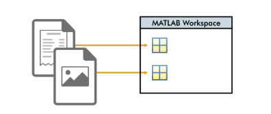
In all MATLAB image processing workflows, the first step is importing images into the MATLAB workspace.
Once there, you can use MATLAB functions to display, process, and classify the images.
You can import an image into memory and assign it to a variable in the MATLAB workspace for later manipulation, display, and export. A = imread("imgFile.jpg"); Ending the line with a semicolon stops MATLAB from displaying the values stored in A, which is helpful since images typically contain millions of values.
I = imread("IMG_001.jpg");
In this training, you'll work with a mix of receipt and non-receipt images. The file names don't indicate if an image is a receipt image or not, but you can find out by displaying the image. Image data stored in a variable A can be displayed using the imshow function.
imshow(A)
imshow(I)
I2 = imread("IMG_002.jpg");
imshow(I2)
You often want to view multiple images. For example, you might want to compare an image and a modified version of that image.
You can display two images together using the imshowpair function.
imshowpair(A1,A2,"montage")
The "montage" option places the images A1 and A2 side-by-side, with A1 on the left and A2 on the right.
imshowpair(I,I2,"montage")
When you're done processing an image in MATLAB, you can save it to a file. The function imwrite exports data stored in the MATLAB workspace to an image file.
imwrite(imgData,"img.jpg")
The output file format is automatically identified based on the file extension.
Try using imwrite to export I as a PNG file. Then use imread to load the image file into a new variable, and display it.
imwrite(I,"myImage.png")
Inew = imread("myImage.png");
imshow(Inew)
Remember that you can execute your script by clicking the Run or Run Section button in the MATLAB Toolstrip. When you're finished practicing, you may move on to the next section.
2.Grayscale and Color Images
Color planes in receipt images
While receipts contain mostly grayscale colors, receipt images are still stored with three color planes like other color images. Like sunlight, which is composed of a full spectrum of colors, the color planes combine to create bright white paper.
Extract Color Planes and Intensity Values
Many image processing techniques are affected by image size. The images you'll be classifying all have the same size: 600 pixels high and 400 pixels wide. You can find the size of an array using the size function.
sz = size(A)
The first value returned by size is the number of rows in the array, which corresponds to the height of the image. The second value is the number of columns in the array, which corresponds to the width of the image.
I = imread("IMG_003.jpg");
imshow(I)
sz = size(I)
Did the size of the array match the size of the image in pixels? Almost. You probably noticed that there was an additional value returned by the size function: 3. That's because the imported image is a color image, and so it needs a third dimension to store the red, green, and blue color planes. You can access individual color planes of an image by indexing into the third dimension. For example, you can extract the green (second) color plane using the value 2 as the third index.
Ig = I(:,:,2);
R = I(:,:,1);
imshow(R)
Most images use the unsigned 8-bit integer (uint8) data type, which stores integers from 0 to 255. Bright or brightly colored images contain pixel intensity values near 255 in one or more color planes.
The red plane of this receipt image has some pretty bright areas. Do you think it will reach the maximum value of 255?
You can find the largest value in an array using the max function.
Amax = max(A,[],"all")
Using the "all" option finds the maximum across all values in the array. The brackets are required; they are placeholders for an unused input.
Rmax = max(R,[],"all")
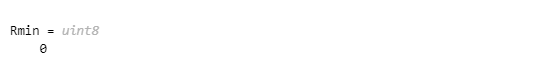
Dark areas, like receipt text, contain values close to zero. Based on the image of the red plane from Task 3, do you think the red plane has any elements with a value of 0?
You can find the smallest value in an array using the min function.
Amin = min(A,[],"all")
Rmin = min(R,[],"all")
Many common tasks can be completed more quickly using functions in Image Processing Toolbox. For example, if you want to extract all three color planes of an image array, you can use imsplit instead of indexing into each plane individually.
[R,G,B] = imsplit(A);
You can display all three color planes at once using montage.
montage({R,G,B})
Try using imsplit to extract the color planes of I. Display all three color planes using montage.
Convert from Color to Grayscale
Why convert to grayscale?
When loaded into memory, a grayscale image occupies a third of the space required for an RGB image.
Because a grayscale image has a third of the data, it requires less computational power to process and can reduce computation time.
A grayscale image is conceptually simpler than an RGB image, so developing an image processing algorithm can be more straightforward when working with grayscale.
In receipt images, like the one shown below, little information is lost when converting to grayscale. The essential characteristics, like the dark text and bright paper, are preserved.
On the other hand, if you wanted to classify the produce visible in the background, the color planes would be essential. After converting to grayscale, it's hard to see the broccoli, let alone classify it.
The algorithm that you’ll implement in this training is built around identifying text, so color is not necessary. Converting the images to grayscale eliminates color and helps the algorithm focus on the black and white patterns found in receipts.
You can convert an image to grayscale using the im2gray function.
Ags = im2gray(A);
I = imread("IMG_002.jpg");
imshow(I)
gs = im2gray(I);
imshow(gs)
Did you notice that the purple color of the receipt text is lost during the conversion to grayscale? However, since not all receipts have purple text, the purple values aren't useful in a classification algorithm.
This negligible loss of information has an upside: gs is one third the size of I, having only two dimensions instead of three. You can verify this with the size function.
sz = size(gs)
The grayscale image created by im2gray is a single plane of intensity values. The intensity values are computed as a weighted sum of the RGB planes, as described here.
If you’ll be needing your converted grayscale images later, you can save them to a file. Try using imwrite to save gs to the file gs.jpg.
3.Contrast Adjustment
Contrast and Intensity Histograms
Even though these two receipt images are grayscale, the contrast is different.
If you are analyzing a set of images, normalizing the brightness can be an important preprocessing step, especially for identifying the black and white patterns of text in receipt images.
An intensity histogram separates pixels into bins based on their intensity values. Dark images, for example, have many pixels binned in the low end of the histogram. Bright regions have pixels binned at the high end of the histogram.
The histogram often suggests where simple adjustments can be made to improve the definition of image features. Do you notice any adjustments that could be made to the receipt image so that the text is easier to identify?
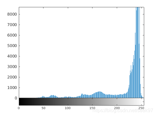
One of the essential identifying features of a receipt image is text. Receipt images should have good contrast so that the text stands out from the paper background. You can investigate the contrast in an image by viewing its intensity histogram using the imhist function.
imhist(I)
If the histogram shows pixels binned mainly at the high and low ends of the spectrum, the receipt has good contrast. If not, it could probably benefit from a contrast adjustment.
Did the histogram of gs suggest high contrast between the text and receipt paper, or do you believe it could use an adjustment?
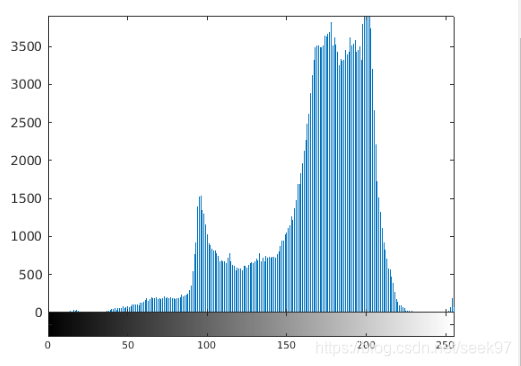
A second image, gs2, is displayed in the script. Does it appear washed out? While a visual inspection can be useful, it’s often easier to assess the contrast by viewing the histogram.
imhist(gs2)
gs2对比度高相对较低
The intensity histogram of gs2 shows lower contrast between the text and the background. Most of the dark pixels have intensity values around 100, and not many bright pixels have intensity values above 200. That means the contrast is about half of what it could be if the image used the full intensity range (0 to 255). Increasing image contrast brightens light pixels and augments dark pixels. You can use the imadjust function to adjust the contrast of a grayscale image automatically.
You can increase the light sensitivity of a digital camera sensor to improve the brightness of a picture taken in low light. Many modern digital cameras (including mobile phone cameras) automatically increase the ISO in dim light. However, this increase in sensitivity amplifies noise picked up by the sensor, leaving the image grainy (shown on the left).
Images taken in low light often become noisy due to the increase in camera sensitivity required to capture the image. This noise can interfere with receipt identification by polluting regions in the binarized image. To reduce the impact of this noise on the binary image, you can preprocess the image with an averaging filter. Use the fspecial function to create an n-by-n averaging filter. F = fspecial("average",n)
I = imread("IMG_007.jpg");
gs = im2gray(I);
gs = imadjust(gs);
BW = imbinarize(gs,"adaptive","ForegroundPolarity","dark");
imshowpair(gs,BW,"montage")
H = fspecial("average",3)
You can apply a filter F to an image I by using the imfilter function.
You may have noticed that filtering introduced an unwanted dark outline to the binary image. That's because the default setting of imfilter sets pixels outside the image to zero. To adjust this behavior, use the "replicate" option. Ifltr = imfilter(I,F,"replicate"); Instead of zeros, the "replicate" option uses pixel intensity values on the image border for pixels outside the image.
Receipt images that have a busy background are more difficult to classify because artifacts pollute the row sum. To mitigate this issue, you can isolate the background and then remove it by subtraction.
In a receipt image, the background is anything that is not text, so isolating the background can be interpreted as removing the text. One way to remove text from an image is to use morphological operations.
A morphological closing operation emphasizes the bright paper and removes the dark text.
Background Subtraction(Remove the Background from a Receipt Image)
In a receipt image, the background is anything that is not text. By using a structuring element larger than a typical letter, each "window" captures what's behind the text and not the text itself. Structuring elements are created using the strel function. SE = strel("diamond",5) The code above defines SE as a diamond-shaped structuring element with radius 5 pixels (the distance from the center to the points of the diamond).
I = imread("IMG_001.jpg");
gs = im2gray(I);
gs = imadjust(gs);
H = fspecial("average",3);
gs = imfilter(gs,H,"replicate");
BW = imbinarize(gs,"adaptive","ForegroundPolarity","dark");
imshowpair(gs,BW,"montage")
SE=strel('disk',8)
The foreground (the text) is dark, and the background is bright. Closing the image will emphasize and connect the brighter background, removing the thin dark lettering. Larger background objects, like the thumb, will remain. The final result: an image of the background without the text.
To perform a closing operation on an image I with structuring element SE, use the imclose function.
Iclosed = imclose(I,SE);
Ibg=imclose(gs,SE);
imshow(Ibg)
Now that you've isolated the background Ibg, you can remove it from gs. In general, you can remove one image from another by subtracting it. Isub = I2 - I1;
Because imclose emphasizes brightness in an image, the background image Ibg has higher intensities than gs. Subtracting Ibg from gs would result in negative intensities.
To avoid negative intensities, subtract gs from Ibg.
gsSub = Ibg - gs;
imshow(gsSub)
Inverting a binary image
A binary image is composed of 0s and 1s. In logical terms, 0 = false and 1 = true. The logical NOT operator (~) reverses the logical state (true becomes false and vice versa). You can use the ~ operator to invert a binary image, which changes all 1s to 0s, and vice versa.
Did you notice anything strange about gsSub?
The subtraction in the previous step inverted the intensities, so the text appears white and the background black. To restore the original order, you need to invert the image again.
First, generate the binary image using imbinarize. Then invert the result using the NOT operator (~).
BWsub = ~imbinarize(gsSub);
imshow(BWsub)
Notice that with good preprocessing, adaptive thresholding wasn't needed. The binarized image BWsub fully captures the text and little else.
Try computing the row sums for the binary images BW and BWsub. Compare the row sums by plotting them on the same axes. Are there notable improvements?
The sequence of operations used here is very common: closing an image, then subtracting the original image from the closed image. It's known as the "bottom hat transform," and you can use the imbothat function in MATLAB to perform it. Try applying imbothat to gs using the structuring element SE.
BW = imbothat(gs,SE);
BW2 = imbothat(gs,SE);
imshow(BW2)
Binary Morphology
Enhancing text patterns
The process from the previous section doesn't remove the grid in the background of this receipt. The grid pattern is too thin to be included in the background generated by the closing operation.
Morphological operations are useful not only for removing features from an image but for augmenting features. You can use morphology to enhance the text in the binary image and improve the row sum signal.
Morphological opening expands the dark text regions, while closing diminishes them. Increasing the size of the structuring element increases these effects.
To enhance a particular shape in an image, create a structural element in the shape of what you want to enhance. Here, each row of text should become a horizontal stripe, which looks like a short, wide rectangle.
You can create a rectangular structuring element using strel with a size array in the format [height width]. SE = strel("rectangle",[10 20]);
To determine the size of the rectangle, you can use features of a typical receipt. The rectangle should be short enough that the white space between rows of text is preserved, and it should be wide enough to connect adjacent letters.
To isolate the background, you wanted to eliminate the dark text by emphasizing the bright regions. To do this, you used imclose to close the image.
Here, you want to emphasize the dark text instead, so you need to perform the opposite operation and open the image using imopen. Iopened = imopen(I,SE);
Using imopen with a wide rectangular structuring element turns lines of text into black horizontal stripes, which augments the valleys in the row sum signal.
BWstripes=imopen(BW,SE);
imshow(BWstripes)
You can analyze whether or not the opening operation has improved the image processing algorithm by plotting the row sum.
S = sum(BWstripes,2);
plot(S)
The improvement becomes more noticeable if you plot the original row sum signal alongside the opened image row sum.
Sbw = sum(BW,2);
hold on
plot(Sbw)
hold off
The text rows generate more pronounced valleys after being enhanced with the opening operation. There is also little to no loss of row definition from the closing operation because the rectangular structuring element was only three pixels high.
By using a very wide rectangular structuring element, there is a risk of amplifying valleys and peaks in the row sums of non-receipt images, which could lead to misclassifications. This risk is acceptable as long as the amplified row sum pattern in receipt images is more pronounced than the unwanted amplification in non-receipt images.
Classification and Batch progressing
Developing a Metric for Receipt Detection:Find Local Minima in a Signal
In general, the row sums of receipt images are visually distinct from the row sums of non-receipt images. The alternating rows of white space and dark text produce characteristic oscillations for receipt images that are absent from other images.
The helper function processImage has been added to the live script to process an image using the algorithm you developed in the previous chapters. All you have to do is adjust the dropdown to load and process an image.
I = imread('testimages/IMG_003.jpg'); % Load an image
[S,BW,BWstripes] = processImage(I); % Process the image to obtain a signal
montage({I,BW,BWstripes}) % Show the image

function [signal,Ibw,stripes] = processImage(img)
    % This function processes an image using the algorithm
    % developed in previous chapters.

    gs = im2gray(img);
    gs = imadjust(gs);

    H = fspecial("average",3);
    gssmooth = imfilter(gs,H,"replicate");

    SE = strel("disk",8);
    Ibg = imclose(gssmooth, SE);
    Ibgsub =  Ibg - gssmooth;
    Ibw = ~imbinarize(Ibgsub);

    SE = strel("rectangle",[3 25]);
    stripes = imopen(Ibw, SE);

    signal = sum(stripes,2);

end
Adding Interactive Tasks to a Live Script
You can add an interactive task to a live script by selecting the Live Editor tab in the MATLAB Toolstrip and then navigating to the desired task.
To automate the receipt classification process, you need a way to identify which images have the row sum oscillations associated with text. Each oscillation contains a peak region (white space) and a valley region (text).
You can use the Find Local Extrema interactive task to identify local minima or maxima in a signal automatically.
The number of minima identified by the task is displayed in the title of the associated plot.
Notice that with the default settings of the Find Local Extrema task, there are many shallow minima identified that don't correspond to rows of text. You can change this by modifying the task parameters so that only prominent minima are found.
Developing a Metric for Receipt Detection:Apply the Classification Metric to an Image
To complete the receipt classification algorithm, you need to count the number of minima in the row sum signal and define a cutoff value that separates receipts from non-receipts.
The array minIndices generated by the Find Local Extrema task is a logical array indicating the locations of the minima. Where a minimum is found, minIndices contains the value 1. Otherwise, it contains the value 0.
You can count the number of minima using the nnz function, which counts the number of nonzero entries in an array. nnz([8 0 7 5 3 0])
The syntax above returns the value 4 since the array has four nonzero elements.
I = imread('testimages/IMG_001.jpg'); % Load an image
[S,BW,BWstripes] = processImage(I); % Process the image to obtain a signal
montage({I,BW,BWstripes}) % Show the image

function [signal,Ibw,stripes] = processImage(img)
    % This function processes an image using the algorithm
    % developed in previous chapters.

    gs = im2gray(img);
    gs = imadjust(gs);

    H = fspecial("average",3);
    gssmooth = imfilter(gs,H,"replicate");

    SE = strel("disk",8);
    Ibg = imclose(gssmooth, SE);
    Ibgsub =  Ibg - gssmooth;
    Ibw = ~imbinarize(Ibgsub);

    SE = strel("rectangle",[3 25]);
    stripes = imopen(Ibw, SE);

    signal = sum(stripes,2);

end
Now you need to define a cutoff value so the algorithm can classify an image as either a receipt or non-receipt.
Based on observations of the available images, 9 or more minima indicates a receipt.
isReceipt = nMin >= 9
Batch Processing with Image Datastores: (2/3) Create an Image Datastore
You've created an algorithm that reads a single image and classifies it. In practice, you’ll have multiple images to process. Image datastores are convenient for locating and accessing multiple image files.
The imageDatastore function creates an image datastore for all the image files in a folder, but won't load them into memory until they are requested.
ds = imageDatastore("localFolder")
ds = imageDatastore("testimages")
You can access the datastore's properties by using a period (.). ds.Folders
The above code accesses the Folders property of the datastore ds.
You can use the numel function to find the total number of elements in an array.
nFiles = numel(dataFilenames)
reusult:
nFiles=18
Batch Processing with Image Datastores: Read and Classify an Image
The readimage function loads the nth image from an image datastore into the MATLAB workspace. img = readimage(ds,n);
ds = imageDatastore("testimages");
I = readimage(ds,1);
imshow(I)
isReceipt = classifyImage(I)

function isReceipt = classifyImage(I)
    % This function processes an image using the algorithm developed in
    % previous chapters and classifies the image as receipt or non-receipt

    % Processing
    gs = im2gray(I);
    gs = imadjust(gs);

    mask = fspecial("average",3);
    gsSmooth = imfilter(gs,mask,"replicate");

    SE = strel("disk",8);
    Ibg = imclose(gsSmooth, SE);
    Ibgsub =  Ibg - gsSmooth;
    Ibw = ~imbinarize(Ibgsub);

    SE = strel("rectangle",[3 25]);
    stripes = imopen(Ibw, SE);

    signal = sum(stripes,2);

    % Classification
    minIndices = islocalmin(signal,"MinProminence",70,"ProminenceWindow",25);
    Nmin = nnz(minIndices);
    isReceipt = Nmin >= 9;

end
Course Example - Extract Images Containing Receipts
With all the image files readily accessible in the datastore ds, you can load and classify every image with just a few lines of code.
You can use a for loop to loop through the n images in a datastore. for k = 1:n ... end
Inside the loop, you can load each image using readimage and classify it using the local function classifyImage.
ds = imageDatastore("testimages");
nFiles = numel(ds.Files);
isReceipt = false(1,nFiles);

for k = 1:nFiles
    I = readimage(ds,k);
    isReceipt(k) = classifyImage(I);
end

function isReceipt = classifyImage(I)
    % This function processes an image using the algorithm developed in
    % previous chapters and classifies the image as receipt or non-receipt

    % Processing
    gs = im2gray(I);
    gs = imadjust(gs);

    H = fspecial("average",3);
    gssmooth = imfilter(gs,H,"replicate");

    SE = strel("disk",8);
    Ibg = imclose(gssmooth, SE);
    Ibgsub =  Ibg - gssmooth;
    Ibw = ~imbinarize(Ibgsub);

    SE = strel("rectangle",[3 25]);
    stripes = imopen(Ibw, SE);

    signal = sum(stripes,2);

    % Classification
    minIndices = islocalmin(signal,"MinProminence",70,"ProminenceWindow",25);
    nMin = nnz(minIndices);
    isReceipt = nMin >= 9;

end
If you want to display the images classified as receipts, you'll need their file names.
You can use the logical array isReceipt as an index to extract the file names of the images classified as receipts. ds.Files(isReceipt)
receiptFiles = ds.Files(isReceipt);
You can display a collection of images by passing their file names to the montage function. montage(imageFileNames)