目录
开发环境
0 项目准备
1 数据集准备
2 数据预处理
3 构建模型
4 模型训练及验证
5 模型部署
6 项目地址
开发环境
作者:嘟粥yyds
时间:2023年8月25日
集成开发工具:PyCharm Professional 2021.1
集成开发环境:Python 3.10.6
第三方库:tensorflow-gpu==2.10.0、cv2==4.7.0、gevent、functools、logging、requests、os、gradio、matplotlib、random
0 项目准备
该部分主要设置一些项目上的超参数,以便读者能根据自身情况修改这些超参数且依旧能正常运行。
# -*- coding: utf-8 -*-
# @File: settings.py
# @Author: 嘟粥yyds
# @Time: 2023/08/25

# ##########爬虫############

# 图片类别和搜索关键词的映射关系
IMAGE_CLASS_KEYWORD_MAP = {
    'cat': '宠物猫',
    'dog': '宠物狗',
    'mouse': '宠物鼠',
    'rabbit': '宠物兔'
}
# 图片保存根目录
IMAGES_ROOT = './images'
# 爬虫每个类别下载多少页图片
SPIDER_DOWNLOAD_PAGES = 20

# #########数据###########

# 每个类别选取的图片数量
SAMPLES_PER_CLASS = 305
# 参与训练的类别
CLASSES = ['cat', 'dog', 'mouse', 'rabbit']
# 参与训练的类别数量
CLASS_NUM = len(CLASSES)
# 类别->编号的映射
CLASS_CODE_MAP = {
    'cat': 0,
    'dog': 1,
    'mouse': 2,
    'rabbit': 3
}
# 编号->类别的映射
CODE_CLASS_MAP = {
    0: '猫',
    1: '狗',
    2: '鼠',
    3: '兔'
}
# 随机数种子
RANDOM_SEED = 13  # 四个类别时样本较为均衡的随机数种子
# RANDOM_SEED = 19  # 三个类别时样本较为均衡的随机数种子
# 训练集比例
TRAIN_DATASET = 0.6
# 开发集比例
DEV_DATASET = 0.2
# 测试集比例
TEST_DATASET = 0.2
# mini_batch大小
BATCH_SIZE = 16
# imagenet数据集均值
IMAGE_MEAN = [0.485, 0.456, 0.406]
# imagenet数据集标准差
IMAGE_STD = [0.299, 0.224, 0.225]

# #########训练#########

# 学习率
LEARNING_RATE = 0.001
# 训练epoch数
TRAIN_EPOCHS = 30
# 保存训练模型的路径
MODEL_PATH = './model.h5'
1 数据集准备
本文不使用任何公开数据集完成该任务,而是通过网络爬虫从网络上爬取需要的数据集素材,再经过人工筛选后形成最后用于训练、验证和测试的数据集。
对于爬虫而言,搜索引擎的选择十分重要。而目前搜索引擎用的比较多的无非两种——Google和百度。我分别使用Google和百度进行了图片搜索,发现百度的搜索结果远不如Google准确,于是就选择了Google,所以我的爬虫代码是基于Google编写的,运行我的爬虫代码需要你的网络能够访问Google。若你的网络不能访问Google,可以考虑自行实现基于百度的爬虫程序,逻辑都是相通的。
由于想让项目更加轻量级一些,故没有使用scrapy框架。爬虫使用requests+beautifulsoup4实现,并发使用gevent实现。
# -*- coding: utf-8 -*-
# @File: spider.py
# @Author: 嘟粥yyds
# @Time: 2023/08/25

from gevent import monkey

monkey.patch_all()  # 使整个程序能够利用gevent的协程特性
import functools
import logging
import os
from bs4 import BeautifulSoup
from gevent.pool import Pool
import requests
import settings

# 设置日志输出格式
logging.basicConfig(format='%(asctime)s - %(pathname)s[line:%(lineno)d] - %(levelname)s: %(message)s',
                    level=logging.INFO)

# 搜索关键词字典
keywords_map = settings.IMAGE_CLASS_KEYWORD_MAP

# 图片保存根目录
images_root = settings.IMAGES_ROOT
# 每个类别下载多少页图片
download_pages = settings.SPIDER_DOWNLOAD_PAGES
# 图片编号字典,每种图片都从0开始编号,然后递增
images_index_map = dict(zip(keywords_map.keys(), [0 for _ in keywords_map]))
# 图片去重器
duplication_filter = set()

# 请求头
headers = {
    'accept-encoding': 'gzip, deflate, br',
    'accept-language': 'zh-CN,zh;q=0.9',
    'user-agent': 'Mozilla/5.0 (Linux; Android 4.0.4; Galaxy Nexus Build/IMM76B) AppleWebKit/537.36 (KHTML, like Gecko) Chrome/46.0.2490.76 Mobile Safari/537.36',
    'accept': '*/*',
    'referer': 'https://www.google.com/',
    'authority': 'www.google.com',
}


# 重试装饰器
def try_again_while_except(max_times=3):
    """
    当出现异常时,自动重试。
    连续失败max_times次后放弃。
    """

    def decorator(func):
        @functools.wraps(func)
        def wrapper(*args, **kwargs):
            error_cnt = 0
            error_msg = ''
            while error_cnt < max_times:
                try:
                    return func(*args, **kwargs)
                except Exception as e:
                    error_msg = str(e)
                    error_cnt += 1
            if error_msg:
                logging.error(error_msg)

        return wrapper

    return decorator


@try_again_while_except()
def download_image(session, image_url, image_class):
    """
    从给定的url中下载图片,并保存到指定路径
    """
    # 下载图片
    resp = session.get(image_url, timeout=20)
    # 检查图片是否下载成功
    if resp.status_code != 200:
        raise Exception('Response Status Code {}!'.format(resp.status_code))
    # 分配一个图片编号
    image_index = images_index_map.get(image_class, 0)
    # 更新待分配编号
    images_index_map[image_class] = image_index + 1
    # 拼接图片路径
    image_path = os.path.join(images_root, image_class, '{}.jpg'.format(image_index))
    # 保存图片
    with open(image_path, 'wb') as f:
        f.write(resp.content)
    # 成功写入了一张图片
    return True


@try_again_while_except()
def get_and_analysis_google_search_page(session, page, image_class, keyword):
    """
    使用google进行搜索,下载搜索结果页面,解析其中的图片地址,并对有效图片进一步发起请求
    """
    logging.info('Class:{} Page:{} Processing...'.format(image_class, page + 1))
    # 记录从本页成功下载的图片数量
    downloaded_cnt = 0
    # 构建请求参数
    params = (
        ('q', keyword),  # 查询关键词
        ('tbm', 'isch'),  # 搜索媒体类型:图片
        ('async', '_id:islrg_c,_fmt:html'),  # 使用异步模式
        ('asearch', 'ichunklite'),  # 使用高级搜索
        ('start', str(page * 100)),  # Google每页大概显示100张图片
        ('ijn', str(page)),  # 搜索结果的页面索引
    )
    # 进行搜索
    resp = requests.get('https://www.google.com/search', params=params, timeout=20)
    # 解析搜索结果
    bsobj = BeautifulSoup(resp.content, 'lxml')
    divs = bsobj.find_all('div', {'class': 'islrtb isv-r'})
    for div in divs:
        image_url = div.get('data-ou')
        # 只有当图片以'.jpg','.jpeg','.png'结尾时才下载图片
        if image_url.endswith('.jpg') or image_url.endswith('.jpeg') or image_url.endswith('.png'):
            # 过滤掉相同图片
            if image_url not in duplication_filter:
                # 使用去重器记录
                duplication_filter.add(image_url)
                # 下载图片
                flag = download_image(session, image_url, image_class)
                if flag:
                    downloaded_cnt += 1
    logging.info('Class:{} Page:{} Done. {} images downloaded.'.format(image_class, page + 1, downloaded_cnt))


def search_with_google(image_class, keyword):
    """
    通过google下载数据集
    """
    # 创建session对象
    session = requests.session()
    session.headers.update(headers)
    # 每个类别下载20页数据
    for page in range(download_pages):
        get_and_analysis_google_search_page(session, page, image_class, keyword)


def run():
    # 首先,创建数据文件夹
    if not os.path.exists(images_root):
        os.mkdir(images_root)
    for sub_images_dir in keywords_map.keys():
        # 对于每个图片类别都创建一个单独的文件夹保存
        sub_path = os.path.join(images_root, sub_images_dir)
        if not os.path.exists(sub_path):
            os.mkdir(sub_path)
    # 开始下载,这里使用gevent的协程池进行并发
    pool = Pool(len(keywords_map))
    for image_class, keyword in keywords_map.items():
        pool.spawn(search_with_google, image_class, keyword)
    pool.join()


if __name__ == '__main__':
    run()
该爬虫使用Google进行图片搜索,每个宠物搜索20页,下载其中的所有图片。当爬虫运行完成后,项目下会多出一个images文件夹,点进去有四个子文件夹,分别为cat、dog、mouse、rabbit。其中每一个子文件夹里面是对应类别的宠物图片。
其中猫图片580+张,狗图片570+张,鼠图片390+张,兔图片480+张。大约花二十多分钟时间,对爬取下来的所有图片进行筛选,剔除其中不符合要求的图片。注意,这一步是必做的,而且要认真对待。(这一步做的好可以使得最后模型的准确率提升8-10个百分点,博主亲身经历)
进行一轮筛选后,剩下图片张数:
| 宠物 |
图片数量 |
| 猫 |
435 |
| 狗 |
468 |
| 鼠 |
305 |
| 兔 |
434 |
考虑各类别样本均衡的问题,无非是过采样和欠采样。因为是图片数据,也可以使用数据增强的手段,为图片数量较少的类别生成一些图片,使样本数量均衡。但出于如下原因考虑,我直接做了欠采样,即每个类别只选取了305张样本:
使用数据增强的话,需要在原图片的基础上,重新生成一份数据集。使用数据增强后,样本数量比较多,无法同时读取到内存里面,只能写个生成器,处理哪一部分的时候,实时从硬盘读取。这个弊端还是很明显的,频繁读取硬盘会拖慢训练速度。
当然,可想而知,使用数据增强(在这里,数据增强可以作为一种过采样的方式)使数据样本都达到468,训练的效果肯定会更好,能好多少就不知道了。相较于我选择的方案复杂,读者若有兴趣可自行实现。
2 数据预处理
由于很多经典的模型接收的输入格式都为(None,224,224,3),由于我们的样本较少,不可避免地需要用到迁移学习,所以我们的数据格式与经典模型保持一致,也使用(None,224,224,3),下面是预处理过程:
# -*- coding: utf-8 -*-
# @File: data.py
# @Author: 嘟粥yyds
# @Time: 2023/08/25

import os
import random
import tensorflow as tf
import settings

# 每个类别选取的图片数量
samples_per_class = settings.SAMPLES_PER_CLASS
# 图片根目录
images_root = settings.IMAGES_ROOT
# 类别->编码的映射
class_code_map = settings.CLASS_CODE_MAP

# 我们准备使用经典网络在imagenet数据集上的与训练权重,所以归一化时也要使用imagenet的平均值和标准差
image_mean = tf.constant(settings.IMAGE_MEAN)
image_std = tf.constant(settings.IMAGE_STD)


def normalization(x):
    """
    对输入图片x进行归一化,返回归一化的值
    """
    return (x - image_mean) / image_std


def train_preprocess(x, y):
    """
    对训练数据进行预处理。
    注意,这里的参数x是图片的路径,不是图片本身;y是图片的标签值
    """
    # 读取图片
    x = tf.io.read_file(x)
    # 解码成张量
    x = tf.image.decode_jpeg(x, channels=3)
    # 将图片缩放到[244,244],比输入[224,224]稍大一些,方便后面数据增强
    x = tf.image.resize(x, [244, 244])
    # 随机决定是否左右镜像
    if random.choice([0, 1]):
        x = tf.image.random_flip_left_right(x)
    # 随机从x中剪裁出(224,224,3)大小的图片
    x = tf.image.random_crop(x, [224, 224, 3])
    # 读完上面的代码可以发现,这里的数据增强并不增加图片数量,一张图片经过变换后,
    # 仍然只是一张图片,跟我们前面说的增加图片数量的逻辑不太一样。
    # 这么做主要是应对我们的数据集里可能会存在相同图片的情况。

    # 将图片的像素值缩放到[0,1]之间
    x = tf.cast(x, dtype=tf.float32) / 255.
    # 归一化
    x = normalization(x)

    # 将标签转成one-hot形式
    y = tf.cast(y, dtype=tf.int32)
    y = tf.one_hot(y, settings.CLASS_NUM)

    return x, y


def dev_preprocess(x, y):
    """
    对验证集和测试集进行数据预处理的方法。
    和train_preprocess的主要区别在于,不进行数据增强,以保证验证结果的稳定性。
    """
    # 读取并缩放图片
    x = tf.io.read_file(x)
    x = tf.image.decode_jpeg(x, channels=3)
    x = tf.image.resize(x, [224, 224])
    # 归一化
    x = tf.cast(x, dtype=tf.float32) / 255.
    x = normalization(x)
    # 将标签转成one-hot形式
    y = tf.cast(y, dtype=tf.int32)
    y = tf.one_hot(y, settings.CLASS_NUM)

    return x, y


# (图片路径,标签)的列表
image_path_and_labels = []
# 排序,保证每次拿到的顺序都一样
sub_images_dir_list = sorted(list(os.listdir(images_root)))
# 遍历每一个子目录
for sub_images_dir in sub_images_dir_list:
    sub_path = os.path.join(images_root, sub_images_dir)
    # 如果给定路径是文件夹,并且这个类别参与训练
    if os.path.isdir(sub_path) and sub_images_dir in settings.CLASSES:
        # 获取当前类别的编码
        current_label = class_code_map.get(sub_images_dir)
        # 获取子目录下的全部图片名称
        images = sorted(list(os.listdir(sub_path)))
        # 随机打乱(排序和置随机数种子都是为了保证每次的结果都一样)
        random.seed(settings.RANDOM_SEED)
        random.shuffle(images)
        # 保留前settings.SAMPLES_PER_CLASS个
        images = images[:samples_per_class]
        # 构建(x,y)对
        for image_name in images:
            abs_image_path = os.path.join(sub_path, image_name)
            image_path_and_labels.append((abs_image_path, current_label))
# 计算各数据集样例数
total_samples = len(image_path_and_labels)  # 总样例数
train_samples = int(total_samples * settings.TRAIN_DATASET)  # 训练集样例数
dev_samples = int(total_samples * settings.DEV_DATASET)  # 开发集样例数
test_samples = total_samples - train_samples - dev_samples  # 测试集样例数
# 打乱数据集
random.seed(settings.RANDOM_SEED)
random.shuffle(image_path_and_labels)
# 将图片数据和标签数据分开,此时它们仍是一一对应的
x_data = tf.constant([img for img, label in image_path_and_labels])
y_data = tf.constant([label for img, label in image_path_and_labels])
# 开始划分数据集
# 训练集
train_db = tf.data.Dataset.from_tensor_slices((x_data[:train_samples], y_data[:train_samples]))
# 打乱顺序,数据预处理,设置批大小
train_db = train_db.shuffle(10000).map(train_preprocess).batch(settings.BATCH_SIZE)
# 开发集(验证集)
dev_db = tf.data.Dataset.from_tensor_slices(
    (x_data[train_samples:train_samples + dev_samples], y_data[train_samples:train_samples + dev_samples]))
# 数据预处理,设置批大小
dev_db = dev_db.map(dev_preprocess).batch(settings.BATCH_SIZE)
# 测试集
test_db = tf.data.Dataset.from_tensor_slices(
    (x_data[train_samples + dev_samples:], y_data[train_samples + dev_samples:]))
# 数据预处理,设置批大小
test_db = test_db.map(dev_preprocess).batch(settings.BATCH_SIZE)
3 构建模型
数据已经全部处理完毕,该考虑模型了。首先,我们数据集太小了,直接构建自己的网络并训练,显而易见并不是一个好方案。因为这几种宠物其实挺难区分的,所以模型需要有一定复杂度,才能很好拟合这些数据,但我们的数据又太少了,最后的结果一定是过拟合,所以我们考虑从迁移学习入手。
一般认为,深度卷积神经网络的训练是对数据集特征的一步步抽取的过程,从简单的特征,到复杂的特征。训练好的模型学习到的是对图像特征的抽取方法,所以在 imagenet 数据集上训练好的模型理论上来说,也可以直接用于抽取其他图像的特征,这也是迁移学习的基础。自然,这样的效果往往没有在新数据上重新训练的效果好,但能够节省大量的训练时间,在特定情况下非常有用。而这种特定情况也包括我们面临的这一种——实际问题的数据集过小。
说到迁移学习,我最先想到的是VGG系列,就先用VGG19跑了一次。使用在 imagenet 数据集上预训练的VGG19网络,去除顶部的全连接层,冻结全部参数,使它们在接下来的训练中不会改变。然后加上自己的全连接层,最后的输出层节点为4,对应于我们的四分类问题。开始训练。
模型在训练集上的误差表现还不错,但是在验证集上的准确率基本在70+%。很明显,这个模型发生过拟合了。
于是,我盯上了DenseNet121,它的参数数量只有7M。果然,在一段时间的调优后,模型的性能有了明显的提升,训练集上达到了91%左右,验证集上的accuracy达到了93%左右。对于DenseNet121而言,这个问题已经不再是过拟合问题了,而是欠拟合了。即数据集规模过小。
# -*- coding: utf-8 -*-
# @File: models.py
# @Author: 嘟粥yyds
# @Time: 2023/08/25

import tensorflow as tf
import settings
from tensorflow.keras.utils import plot_model


def my_densenet():
    """
    创建并返回一个基于densenet的Model对象
    """
    # 获取densenet网络,使用在imagenet上训练的参数值,移除头部的全连接网络,池化层使用max_pooling
    densenet = tf.keras.applications.DenseNet121(include_top=False, weights='imagenet', pooling='max')
    # 冻结预训练的参数,在之后的模型训练中不会改变它们
    densenet.trainable = False
    # 构建模型
    model = tf.keras.Sequential([
        # 输入层,shape为(None,224,224,3)
        tf.keras.layers.Input((224, 224, 3)),
        # 输入到DenseNet121中
        densenet,
        # 将DenseNet121的输出展平,以作为全连接层的输入
        tf.keras.layers.Flatten(),
        # 添加BN层
        tf.keras.layers.BatchNormalization(),
        # 随机失活
        tf.keras.layers.Dropout(0.5),
        # 第一个全连接层,激活函数relu
        tf.keras.layers.Dense(512, activation=tf.nn.relu),
        # BN层
        tf.keras.layers.BatchNormalization(),
        # 随机失活
        tf.keras.layers.Dropout(0.5),
        # 第二个全连接层,激活函数relu
        tf.keras.layers.Dense(64, activation=tf.nn.relu),
        # BN层
        tf.keras.layers.BatchNormalization(),
        # 输出层,为了保证输出结果的稳定,这里就不添加Dropout层了
        tf.keras.layers.Dense(settings.CLASS_NUM, activation=tf.nn.softmax)
    ])

    return model


if __name__ == '__main__':
    model = my_densenet()
    model.summary()
    plot_model(model, show_shapes=True, to_file='model.png', dpi=200)
 模型的summary:
Model: "sequential"
_________________________________________________________________
 Layer (type)                Output Shape              Param #
=================================================================
 densenet121 (Functional)    (None, 1024)              7037504

 flatten (Flatten)           (None, 1024)              0

 batch_normalization (BatchN  (None, 1024)             4096
 ormalization)

 dropout (Dropout)           (None, 1024)              0

 dense (Dense)               (None, 512)               524800

 batch_normalization_1 (Batc  (None, 512)              2048
 hNormalization)

 dropout_1 (Dropout)         (None, 512)               0

 dense_1 (Dense)             (None, 64)                32832

 batch_normalization_2 (Batc  (None, 64)               256
 hNormalization)

 dense_2 (Dense)             (None, 4)                 260

=================================================================
Total params: 7,601,796
Trainable params: 561,092
Non-trainable params: 7,040,704
_________________________________________________________________
参数总量7601796个,其中可训练参数561092个 。
4 模型训练及验证
模型和数据都已准备完毕,可以开始训练了。让我们编写一个训练用的脚本:
# -*- coding: utf-8 -*-
# @File: train.py
# @Author: 嘟粥yyds
# @Time: 2023/08/25

import tensorflow as tf
from tensorflow.keras.callbacks import ModelCheckpoint, EarlyStopping, ReduceLROnPlateau, TensorBoard
from data import train_db, dev_db
import models
import settings

# 从models文件中导入模型
model = models.my_densenet()

# 创建 TensorBoard 回调对象
tensorboard_callback = TensorBoard(log_dir='logs', histogram_freq=1, write_graph=True, write_images=True)

# 配置优化器、损失函数、以及监控指标
model.compile(tf.keras.optimizers.Adam(settings.LEARNING_RATE), loss=tf.keras.losses.categorical_crossentropy,
              metrics=['accuracy'])

# 在每个epoch结束后尝试保存模型参数,只有当前参数的val_accuracy比之前保存的更优时,才会覆盖掉之前保存的参数
model_check_point = ModelCheckpoint(filepath=settings.MODEL_PATH, monitor='val_accuracy',
                                    save_best_only=True)

# 创建早停回调对象
early_stopping = EarlyStopping(monitor='val_loss', patience=8, restore_best_weights=True)

# 创建学习率减少回调对象
lr_decay = ReduceLROnPlateau(monitor='val_loss', factor=0.1, patience=3, min_lr=1e-6)

# 使用高级接口进行训练
model.fit(train_db, epochs=settings.TRAIN_EPOCHS, validation_data=dev_db,
          callbacks=[model_check_point, early_stopping, lr_decay, tensorboard_callback])
现在,我们可以运行脚本进行训练了,最优的参数将被保存在settings.MODEL_PATH。训练完成后,我们需要调用以下验证脚本,验证下模型在验证集和测试集上的表现:
# -*- coding: utf-8 -*-
# @File    : eval.py
# @Author  : 嘟粥yyds
# @Time    : 2023/08/25

import tensorflow as tf
from data import dev_db, test_db
from models import my_densenet
import settings

# 创建模型
model = my_densenet()
# 加载参数
model.load_weights(settings.MODEL_PATH)
# 因为想用tf.keras的高级接口做验证,所以还是需要编译模型
model.compile(tf.keras.optimizers.Adam(settings.LEARNING_RATE), loss=tf.keras.losses.categorical_crossentropy,
              metrics=['accuracy'])
# 验证集accuracy
print('dev', model.evaluate(dev_db))
# 测试集accuracy
print('test', model.evaluate(test_db))

# 查看识别错误的数据
for x, y in test_db:
    y_pred = model(x)
    y_pred = tf.argmax(y_pred, axis=1).numpy()
    y_true = tf.argmax(y, axis=1).numpy()
    batch_size = y_pred.shape[0]
    for i in range(batch_size):
        if y_pred[i] != y_true[i]:
            print('{} 被错误识别成 {}!'.format(settings.CODE_CLASS_MAP[y_true[i]], settings.CODE_CLASS_MAP[y_pred[i]]))
16/16 [==============================] - 9s 99ms/step - loss: 0.1439 - accuracy: 0.9713
dev [0.1438767910003662, 0.9713114500045776]
16/16 [==============================] - 1s 85ms/step - loss: 0.1606 - accuracy: 0.9549
test [0.16057191789150238, 0.9549180269241333]
猫 被错误识别成 兔!
猫 被错误识别成 鼠!
猫 被错误识别成 狗!
鼠 被错误识别成 兔!
猫 被错误识别成 狗!
兔 被错误识别成 猫!
兔 被错误识别成 猫!
猫 被错误识别成 兔!
狗 被错误识别成 鼠!
猫 被错误识别成 兔!
狗 被错误识别成 兔!
能够看到,模型在验证集上的准确率为97.13%,在测试集上的准确率为95.49%,已经达到我的心里预期了,毕竟使用的数据确实很少。
5 模型部署
该项目的模型部署依旧是借用Gradio进行部署,其优点不言而喻——方便。
import gradio as gr
import tensorflow as tf
import settings
from models import my_densenet
import matplotlib as mpl
mpl.use('TkAgg')
# 导入模型
model = my_densenet()
# 加载训练好的参数
model.load_weights(settings.MODEL_PATH)
def classify_pet_image(input_image):
"""
宠物图片分类接口,上传一张图片,返回此图片上的宠物是哪种类别,概率多少
"""
# 进行数据预处理
# x = tf.image.decode_image(input_image, channels=3)
x = tf.convert_to_tensor(input_image)
x = tf.image.resize(x, (224, 224))
x = x / 255.
x = (x - tf.constant(settings.IMAGE_MEAN)) / tf.constant(settings.IMAGE_STD)
x = tf.reshape(x, (1, 224, 224, 3))
# 预测
y_pred = model(x)
pet_cls_code = tf.argmax(y_pred, axis=1).numpy()[0]
pet_cls_prob = float(y_pred.numpy()[0][pet_cls_code])
pet_cls_prob = '{}%'.format(int(pet_cls_prob * 100))
pet_class = settings.CODE_CLASS_MAP.get(pet_cls_code)
# 格式化输出为纯文本
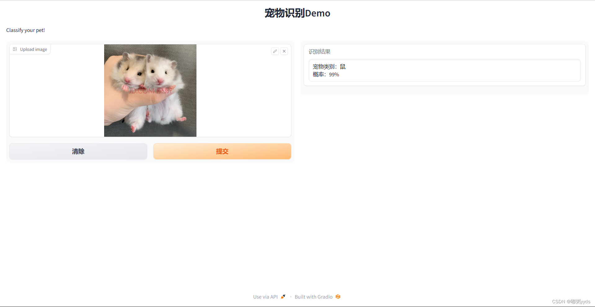
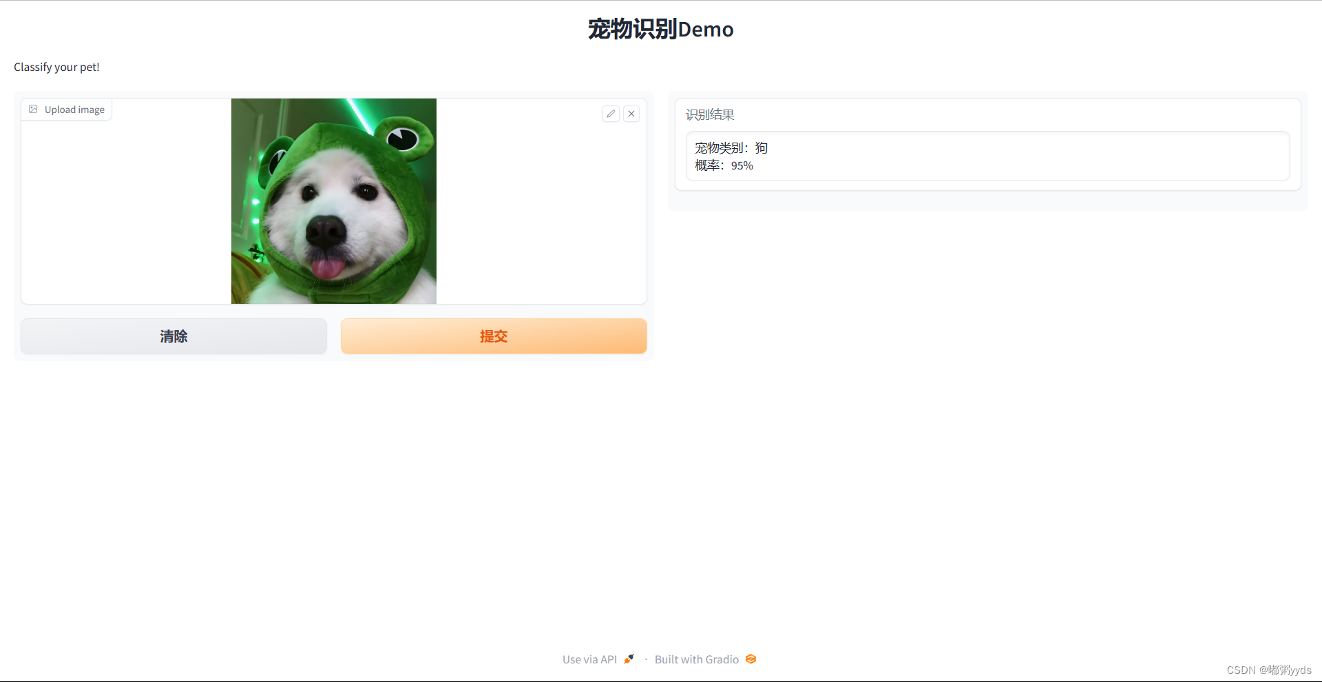
output_text = "宠物类别:{} \n概率:{}".format(pet_class, pet_cls_prob)
return output_text
gr.close_all()
demo = gr.Interface(fn=classify_pet_image,
inputs=[gr.Image(label="Upload image")],
outputs=[gr.Textbox(label="识别结果")],
title="宠物识别Demo",
description="Classify your pet!",
allow_flagging="never"
)
demo.launch(share=True, debug=True, server_port=10055)


6 项目地址
Github:GitHub - 0911duzhou/OpenCV-Pet_Classifer: 基于TensorFlow2实现的宠物识别系统(爬虫、模型训练和调优、模型部署)
若无法访问Github也可在博主的主页资源里下载。