作者 | 密斯特李 编辑 | 汽车人
原文链接:https://zhuanlan.zhihu.com/p/511968459
点击下方卡片,关注“自动驾驶之心”公众号
ADAS巨卷干货,即可获取
点击进入→自动驾驶之心技术交流群
后台回复【IROS2022】获取IROS2022所有自动驾驶方向论文!
0、引子
上期文章介绍了F-LOAM,它重点针对LOAM计算效率问题进行了优化,旨在不影响精度的情况下尽量缩减其对平台算力的需求,使之能够轻量化地部署于算力有限的无人平台上(例如:无人机、移动机器人等)。F-LOAM所采用的优化思路是舍弃LOAM中不必要的laserOodmetry线程并以匀速运动模型估计的位姿预测代替。代码实现整体与A-LOAM一脉相承,除结构优化外在实现细节方面并没有什么差异。
本文介绍的LeGO-LOAM同样是针对LOAM计算效率问题的优化,针对地面移动机器人在室内外环境下运行时的特点,针对性的对LOAM进行优化和改进,实现了一套轻量级的激光雷达SLAM系统。该工作由Shan Tixiao完成,论文LeGO-LOAM: Lightweight and Ground-Optimized LiDAR Odometry and Mapping on Variance Terrain发表于2018年IROS会议,代码源生于LOAM的原始版本,开源于RobustFieldAutonomyLab/LeGO-LOAM,优化版本的代码见facontidavide/LeGO-LOAM-BOR。
相比于F-LOAM, LeGO-LOAM不仅整合了LOAM的系统结构,同时对LOAM中的特征提取、位姿估计计算都进行了优化改进,此外还加入了闭环检测和全局优化,将LOAM这一LO系统构建为完整的SLAM系统,整体工作的创新性和完整性都更加突出。
1、主要创新点及系统架构
1.1 主要创新点
根据论文内容和代码,笔者将这一工作的主要创新点归纳为以下几点:
相较于LOAM的第一个改进:增加基于柱面投影特征分割,对原始点云进行地面点分割和目标聚类。
相较于LOAM的第二个改进:基于分割点云的线面特征提取,从地面点和目标聚类点云中提取线、面特征,特征点更精确。
相较于LOAM的第三个改进:采用两步法实现laserOdometry线程的位姿优化计算,在优化估计精度保持不变的情况下收敛速度极大提升。
相较于LOAM的第四个改进:采用关键帧进行局部地图和全局地图的管理,邻近点云的索引更为便捷。
相较于LOAM的第五个改进:增加基于距离的闭环检测和全局优化,构成完整的激光SLAM解决方案。
1.2 系统架构
LeGO-LOAM的系统架构在其论文中展示的很清晰,ROS的节点关系也能清晰地展示系统各模块间的关系,如下图:
 LeGO-LOAM系统架构
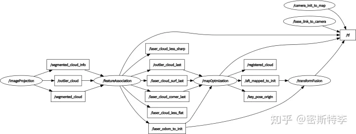 LeGO-LOAM的ROS节点关系图
与LOAM类似,系统整体分为四个部分,对应四个ROS节点,在四个不同进程中运行。不同的是,LeGO-LOAM将LOAM中负责点云特征提取的scanRegistration节点和负责scan-to-scan匹配的laserOdometry节点整合为featureAssociation节点,增加imageProjection节点,同时在mapOptimization节点中开辟闭环检测与全局优化线程。各节点的具体功能如下:
2、主要方法及代码实现
2.1 点云投影与目标分割
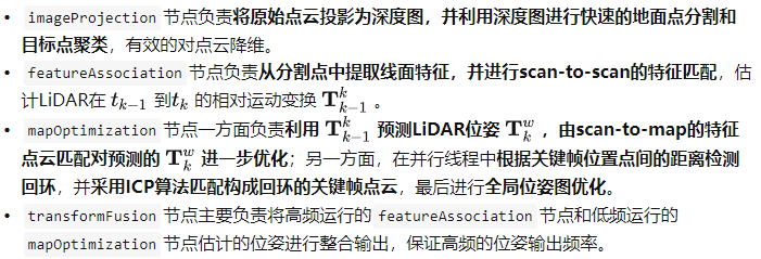
LiDAR直接输出的原始点云是无序的,即无法像图像一样能够明确的知道点云中某一点上下左右的点是哪个,因此在数据处理时通常需要建立树型结构(例如KD树、八叉树)对点云数据进行数据组织和管理。点云投影实际上是一种将无序点云有序化的过程,我们可以直接从投影的点云深度图(depth image 或 range image)中索引到某一点的上下或两侧的点,这也将极大地提高目标分割的效率。
 点云与深度图投影示意图
在LeGO-LOAM代码中,实现部分在imageProjection.cpp中的projectPointCloud()函数中实现,具体说明见代码中注释:
void projectPointCloud(){
        // range image projection
        float verticalAngle, horizonAngle, range;
        size_t rowIdn, columnIdn, index, cloudSize;
        PointType thisPoint;

        cloudSize = laserCloudIn->points.size(); // 点云中点个数

        for (size_t i = 0; i < cloudSize; ++i){ // 逐点计算

            thisPoint.x = laserCloudIn->points[i].x;
            thisPoint.y = laserCloudIn->points[i].y;
            thisPoint.z = laserCloudIn->points[i].z;
            // find the row and column index in the iamge for this point
            if (useCloudRing == true){ // 当LiDAR驱动能够输出scan line信息时,直接读取
                rowIdn = laserCloudInRing->points[i].ring;
            }
            else{ // 否则,需要计算俯仰角
                verticalAngle = atan2(thisPoint.z, sqrt(thisPoint.x * thisPoint.x + thisPoint.y * thisPoint.y)) * 180 / M_PI; // 单位为度
                rowIdn = (verticalAngle + ang_bottom) / ang_res_y; // 计算行号,见公式(1)
            }
            if (rowIdn < 0 || rowIdn >= N_SCAN)
                continue;

            horizonAngle = atan2(thisPoint.x, thisPoint.y) * 180 / M_PI; // 计算列号,见公式(2)

            // 由于atan2返回的是(-pi,pi)的一个值,为了保证正前方在深度图的中间,需要进行如下角度变换。
            columnIdn = -round((horizonAngle-90.0)/ang_res_x) + Horizon_SCAN/2;
            if (columnIdn >= Horizon_SCAN)
                columnIdn -= Horizon_SCAN;

            if (columnIdn < 0 || columnIdn >= Horizon_SCAN)
                continue;
            //
            range = sqrt(thisPoint.x * thisPoint.x + thisPoint.y * thisPoint.y + thisPoint.z * thisPoint.z);
            if (range < sensorMinimumRange) // 舍弃深度小于最小阈值的点
                continue;

            rangeMat.at<float>(rowIdn, columnIdn) = range; // 构建深度图

            thisPoint.intensity = (float)rowIdn + (float)columnIdn / 10000.0;

            index = columnIdn  + rowIdn * Horizon_SCAN; // 深度图像素坐标对应的索引号
            fullCloud->points[index] = thisPoint; // 构建点云
            fullInfoCloud->points[index] = thisPoint;
            fullInfoCloud->points[index].intensity = range; // the corresponding range of a point is saved as "intensity"
        }
    }
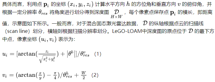
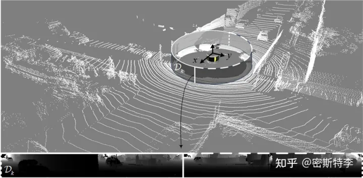
而后,利用投影深度图进行地面点分割。该方法的前提是默认了深度图下部大部分区域为地面点,且由于无人车位于地面上,车载LiDAR的 平面与地面大致水平, 与地面大致垂直。因此,若深度图上两像素点所构成的向量与LiDAR坐标系 平面的夹角很小,则该向量就近似位于地面上。具体实现部分见imageProjection.cpp的groundRemoval()函数,具体说明见代码中的注释:
void groundRemoval(){
        size_t lowerInd, upperInd;
        float diffX, diffY, diffZ, angle;
        // 构建地面点深度图groundMat
        // -1, 深度图中的无效区域
        //  0, 非地面点标记
        //  1, 地面点标记
        for (size_t j = 0; j < Horizon_SCAN; ++j){
            for (size_t i = 0; i < groundScanInd; ++i){

                lowerInd = j + ( i )*Horizon_SCAN; // 当前像素点下方像素的索引号
                upperInd = j + (i+1)*Horizon_SCAN; // 当前像素点上方像素的索引号

                if (fullCloud->points[lowerInd].intensity == -1 ||
                    fullCloud->points[upperInd].intensity == -1){ // 对应像素无深度值
                    // no info to check, invalid points
                    groundMat.at<int8_t>(i,j) = -1;
                    continue;
                }
                // 构建向量
                diffX = fullCloud->points[upperInd].x - fullCloud->points[lowerInd].x;
                diffY = fullCloud->points[upperInd].y - fullCloud->points[lowerInd].y;
                diffZ = fullCloud->points[upperInd].z - fullCloud->points[lowerInd].z;

                angle = atan2(diffZ, sqrt(diffX*diffX + diffY*diffY) ) * 180 / M_PI; // 计算向量与x-y平面的夹角

                if (abs(angle - sensorMountAngle) <= 10){ // sensorMountAngle表示LiDAR安装时与地面的夹角,通俗来说头朝下时夹角为正,头朝上扬起时夹角为负
                    groundMat.at<int8_t>(i,j) = 1;
                    groundMat.at<int8_t>(i+1,j) = 1; // 若夹角小于10°,则将构成向量的两个深度图像素点标记为地面点
                }
            }
        }
        // extract ground cloud (groundMat == 1)
        // mark entry that doesn't need to label (ground and invalid point) for segmentation
        // note that ground remove is from 0~N_SCAN-1, need rangeMat for mark label matrix for the 16th scan
        for (size_t i = 0; i < N_SCAN; ++i){
            for (size_t j = 0; j < Horizon_SCAN; ++j){
                if (groundMat.at<int8_t>(i,j) == 1 || rangeMat.at<float>(i,j) == FLT_MAX){
                    labelMat.at<int>(i,j) = -1;
                }
            }
        }
        if (pubGroundCloud.getNumSubscribers() != 0){
            for (size_t i = 0; i <= groundScanInd; ++i){
                for (size_t j = 0; j < Horizon_SCAN; ++j){
                    if (groundMat.at<int8_t>(i,j) == 1)
                        groundCloud->push_back(fullCloud->points[j + i*Horizon_SCAN]); // 插入地面点点云
                }
            }
        }
    }
地面点分割后,对非地面点进行进一步的目标聚类分割。采用广度优先搜索算法(Breadth-First Search,BFS)在非地面深度图上对所有深度像素进行聚类分割,原则是:某一像素点与其邻域点及LiDAR坐标系原点O构成三角型,另深度值较大的点为A,较小的点为B。当 较大时则认为A和B位于同一目标。分割算法的具体细节可参考文献[1]。LeGO-LOAM中代码实现见imageProjection.cpp的labelComponents(int row, int col)函数:
void labelComponents(int row, int col){
        // use std::queue std::vector std::deque will slow the program down greatly
        float d1, d2, alpha, angle;
        int fromIndX, fromIndY, thisIndX, thisIndY;
        bool lineCountFlag[N_SCAN] = {false};

        queueIndX[0] = row;
        queueIndY[0] = col;
        int queueSize = 1;
        int queueStartInd = 0;
        int queueEndInd = 1;

        allPushedIndX[0] = row;
        allPushedIndY[0] = col;
        int allPushedIndSize = 1;

        while(queueSize > 0){ // BFS搜索的主循环
            // Pop point
            fromIndX = queueIndX[queueStartInd];
            fromIndY = queueIndY[queueStartInd];
            --queueSize;
            ++queueStartInd;
            // Mark popped point
            labelMat.at<int>(fromIndX, fromIndY) = labelCount; // 对目标类别标号
            // Loop through all the neighboring grids of popped grid
            for (auto iter = neighborIterator.begin(); iter != neighborIterator.end(); ++iter){ // 邻域搜索
                // new index
                thisIndX = fromIndX + (*iter).first;
                thisIndY = fromIndY + (*iter).second;
                // index should be within the boundary
                if (thisIndX < 0 || thisIndX >= N_SCAN)
                    continue;
                // at range image margin (left or right side)
                if (thisIndY < 0)
                    thisIndY = Horizon_SCAN - 1;
                if (thisIndY >= Horizon_SCAN)
                    thisIndY = 0;
                // prevent infinite loop (caused by put already examined point back)
                if (labelMat.at<int>(thisIndX, thisIndY) != 0)
                    continue;

                d1 = std::max(rangeMat.at<float>(fromIndX, fromIndY),
                              rangeMat.at<float>(thisIndX, thisIndY)); // 深度较大的点,即A
                d2 = std::min(rangeMat.at<float>(fromIndX, fromIndY),
                              rangeMat.at<float>(thisIndX, thisIndY)); // 深度较小的点,即B
                // 角AOB实际上就是深度图像素点划分时所设定的角度分辨率
                if ((*iter).first == 0)
                    alpha = segmentAlphaX; // 若邻域点为同一行的点,则角AOB为水平方向的角度分辨率
                else
                    alpha = segmentAlphaY; // 若邻域点为同一列的点,则角AOB为垂直方向的角度分辨率

                angle = atan2(d2*sin(alpha), (d1 -d2*cos(alpha))); // 计算角OAB

                if (angle > segmentTheta){ // 若角OAB大于所设阈值,则认为A和B位于同一目标

                    queueIndX[queueEndInd] = thisIndX;
                    queueIndY[queueEndInd] = thisIndY; // 重置搜索起点,以当前邻域点为起点继续搜索
                    ++queueSize;
                    ++queueEndInd;

                    labelMat.at<int>(thisIndX, thisIndY) = labelCount;
                    lineCountFlag[thisIndX] = true;

                    allPushedIndX[allPushedIndSize] = thisIndX;
                    allPushedIndY[allPushedIndSize] = thisIndY;
                    ++allPushedIndSize;
                }
            }
        }

        // check if this segment is valid
        bool feasibleSegment = false;
        if (allPushedIndSize >= 30)
            feasibleSegment = true; // 若当前目标点个数大于30个,则该目标为有效目标
        else if (allPushedIndSize >= segmentValidPointNum){
            // 若不足30但大于所设最小有效阈值,则判断该目标是否跨越足够多的行。若是,则同样标记为有效目标
            // 这一判断是避免一些垂直地面的柱状目标(如:路标杆、树干)因聚类目标点个数过少而被错误的标记为无效
            int lineCount = 0;
            for (size_t i = 0; i < N_SCAN; ++i)
                if (lineCountFlag[i] == true)
                    ++lineCount;
            if (lineCount >= segmentValidLineNum)
                feasibleSegment = true;
        }
        // segment is valid, mark these points
        if (feasibleSegment == true){
            ++labelCount;
        }else{ // segment is invalid, mark these points
            for (size_t i = 0; i < allPushedIndSize; ++i){
                labelMat.at<int>(allPushedIndX[i], allPushedIndY[i]) = 999999; // 无效目标点的标记
            }
        }
    }
2.2 特征提取与激光里程计
LeGO-LOAM采用与LOAM中相同的特征提取方法,即根据邻域点平滑度筛选线和面特征,本文不再赘述。主要区别是LeGO-LOAM特征提取时兼顾了地面分割和目标聚类的结果。筛选出地面点作为平面特征,并从非地面点且有效聚类目标中提取线特征。代码实现参考featureAssociation.cpp的calculateSmoothness()、markOccludedPints()和extractFeatures()等函数。
激光里程计通过scan-to-scan匹配估计LiDAR在到间的相对运动,特征匹配方法与LOAM中相同,唯一区别在于LeGO-LOAM采用两步法实现6自由度的位姿状态估计。根据作者的测试,采用两步法能够在获得相同精度的前提下降低35%的计算时间消耗,大大提升了运算效率。具体而言,先利用地面特征估计相对位姿的俯仰角ry、横滚角rx和z轴平移量三个自由度;而后再利用线特征估计相对位姿的偏航角rz、x轴平移量和y轴平移量。代码实现见featureAssociation.cpp的updateTransformation()函数:
void updateTransformation(){

        if (laserCloudCornerLastNum < 10 || laserCloudSurfLastNum < 100)
            return;

        for (int iterCount1 = 0; iterCount1 < 25; iterCount1++) { // 第一步: 根据地面特征估计三个自由度
            laserCloudOri->clear();
            coeffSel->clear();

            findCorrespondingSurfFeatures(iterCount1);

            if (laserCloudOri->points.size() < 10)
                continue;
            if (calculateTransformationSurf(iterCount1) == false)
                break;
        }

        for (int iterCount2 = 0; iterCount2 < 25; iterCount2++) { // 第二步: 根据线特征估计其余的三个自由度

            laserCloudOri->clear();
            coeffSel->clear();

            findCorrespondingCornerFeatures(iterCount2);

            if (laserCloudOri->points.size() < 10)
                continue;
            if (calculateTransformationCorner(iterCount2) == false)
                break;
        }
    }
通过构建非线性优化方程,采用L-M算法求解相对位姿变换。L-M优化迭代部分的实现在上述代码的calculateTransformationSurf()和 calculateTransformationCorner() 函数中。这里要填一下上一篇文章提到的“采用ceres等优化计算库改进LOAM代码后会产生一定问题”这个坑。在LOAM的优化迭代实现中,引入了退化因子(degeneracy factor)的概念,通过退化因子判断特征退化方向。
那么什么是特征退化?这里我通俗的解释一下:对于点云特征匹配而言,我们将它构建为了一个非线性优化(Nonlinear Optimization)问题,这个非线性优化问题的解是一个六自由度的位姿变换。平行于x-y平面的特征点云可以为估计rx,ry,z提供充足的约束;而平行于z-y和z-x平面的特征点云则可以为估计rz,x,y提供充足的约束。但如果实在一个看不到头尾的长直隧道中,显然平行于平面z-x的点云是严重不足的,导致难以估计x平移量,这就是所谓的退化问题,专业点讲即观测约束在状态空间中是不完备的。对于特征退化因子的理论和推导可以参看LOAM作者Ji Zhang的另一篇论文[2],本文不再深入,若感兴趣的同学比较多我们再单独出一篇解析。具体实现也比较简单,说白了L-M迭代就是在给定初值的基础上增量式地朝着无偏最优估计逼近。若状态空间的某一个方向发现了退化,那就直接不更新这个方向的值就好了。通过将对应状态方向的权阵置0,使这个方向的估计增量不会被加在优化初值上。这里以calculateTransformationCorner()函数为例:
bool calculateTransformationCorner(int iterCount){

        int pointSelNum = laserCloudOri->points.size();

        cv::Mat matA(pointSelNum, 3, CV_32F, cv::Scalar::all(0));
        cv::Mat matAt(3, pointSelNum, CV_32F, cv::Scalar::all(0));
        cv::Mat matAtA(3, 3, CV_32F, cv::Scalar::all(0));
        cv::Mat matB(pointSelNum, 1, CV_32F, cv::Scalar::all(0));
        cv::Mat matAtB(3, 1, CV_32F, cv::Scalar::all(0));
        cv::Mat matX(3, 1, CV_32F, cv::Scalar::all(0));

        float srx = sin(transformCur[0]);
        float crx = cos(transformCur[0]);
        float sry = sin(transformCur[1]);
        float cry = cos(transformCur[1]);
        float srz = sin(transformCur[2]);
        float crz = cos(transformCur[2]);
        float tx = transformCur[3];
        float ty = transformCur[4];
        float tz = transformCur[5];

        float b1 = -crz*sry - cry*srx*srz; float b2 = cry*crz*srx - sry*srz; float b3 = crx*cry; float b4 = tx*-b1 + ty*-b2 + tz*b3;
        float b5 = cry*crz - srx*sry*srz; float b6 = cry*srz + crz*srx*sry; float b7 = crx*sry; float b8 = tz*b7 - ty*b6 - tx*b5;

        float c5 = crx*srz;

        // 利用观测到的线特征构建优化方程的系数矩阵A和残差向量B
        for (int i = 0; i < pointSelNum; i++) {

            pointOri = laserCloudOri->points[i];
            coeff = coeffSel->points[i];

            float ary = (b1*pointOri.x + b2*pointOri.y - b3*pointOri.z + b4) * coeff.x
                      + (b5*pointOri.x + b6*pointOri.y - b7*pointOri.z + b8) * coeff.z;

            float atx = -b5 * coeff.x + c5 * coeff.y + b1 * coeff.z;

            float atz = b7 * coeff.x - srx * coeff.y - b3 * coeff.z;

            float d2 = coeff.intensity;

            matA.at<float>(i, 0) = ary;
            matA.at<float>(i, 1) = atx;
            matA.at<float>(i, 2) = atz;
            matB.at<float>(i, 0) = -0.05 * d2;
        }

        cv::transpose(matA, matAt);
        matAtA = matAt * matA;
        matAtB = matAt * matB;
        cv::solve(matAtA, matAtB, matX, cv::DECOMP_QR); // QR分解法求解 AtAX = AtB

        if (iterCount == 0) {
            cv::Mat matE(1, 3, CV_32F, cv::Scalar::all(0));
            cv::Mat matV(3, 3, CV_32F, cv::Scalar::all(0));
            cv::Mat matV2(3, 3, CV_32F, cv::Scalar::all(0));

            cv::eigen(matAtA, matE, matV); // 对AtA这一对称矩阵进行特征值分解
            matV.copyTo(matV2); // 特征向量,一行对应一个状态方向

            isDegenerate = false;
            float eignThre[3] = {10, 10, 10};
            for (int i = 2; i >= 0; i--) { // 从最小特征值开始
                if (matE.at<float>(0, i) < eignThre[i]) {
                    for (int j = 0; j < 3; j++) {
                        matV2.at<float>(i, j) = 0; // 若出现退化,将这一行置零
                    }
                    isDegenerate = true;
                } else {
                    break;
                }
            }
            matP = matV.inv() * matV2; // 由于AtA是方阵,根据对称对角化定理V^-1 = Vt
        }

        if (isDegenerate) {
            cv::Mat matX2(3, 1, CV_32F, cv::Scalar::all(0));
            matX.copyTo(matX2);
            matX = matP * matX2;
        }

        transformCur[1] += matX.at<float>(0, 0);
        transformCur[3] += matX.at<float>(1, 0);
        transformCur[5] += matX.at<float>(2, 0);

        for(int i=0; i<6; i++){
            if(isnan(transformCur[i]))
                transformCur[i]=0;
        }

        float deltaR = sqrt(
                            pow(rad2deg(matX.at<float>(0, 0)), 2));
        float deltaT = sqrt(
                            pow(matX.at<float>(1, 0) * 100, 2) +
                            pow(matX.at<float>(2, 0) * 100, 2));

        if (deltaR < 0.1 && deltaT < 0.1) { // 判断收敛
            return false;
        }
        return true;
    }
2.3 地图优化
在这一节点中,共并行了3个线程,分别是:
主线程:scan-to-map匹配以优化激光雷达里程计估计结果,采用基于因子图优化的增量式平滑算法(incremental smoothing and mapping,iSAM)进行整体的位姿图优化
分线程:基于距离的闭环检测,对可能产生闭环的关键帧进行ICP配准,获得闭环帧之间的相对变换加入全局位姿图,并采用iSAM进行整体优化
分线程:对点云、轨迹和构建的位姿图网络进行可视化,并保存点云和离散轨迹。
主线程的scan-to-map匹配与LOAM完全一致,主要改进在于局部地图的管理。LOAM中采用栅格图对局部点云进行管理,栅格图大小固定,随着LiDAR的运动而移动。在LeGO-LOAM中则采用基于关键帧的地图管理方式,这种方法的优点一方面是便于全局优化更新,另一方面是能够更加真实的反映LiDAR邻域环境情况,局部地图更丰富;缺点也很显然,内存占用随运行时间而不断增加,占用内存更大。局部地图的构建同样距离判断,具体实现在mapOptimization.cpp的 extractSurroundingKeyFrames()函数中:
surroundingKeyPoses->clear();
            surroundingKeyPosesDS->clear();
         // extract all the nearby key poses and downsample them
         kdtreeSurroundingKeyPoses->setInputCloud(cloudKeyPoses3D); // 利用KD数搜索邻近的关键帧
         kdtreeSurroundingKeyPoses->radiusSearch(currentRobotPosPoint, (double)surroundingKeyframeSearchRadius, pointSearchInd, pointSearchSqDis, 0);
         for (int i = 0; i < pointSearchInd.size(); ++i)
                surroundingKeyPoses->points.push_back(cloudKeyPoses3D->points[pointSearchInd[i]]);
         downSizeFilterSurroundingKeyPoses.setInputCloud(surroundingKeyPoses);
         downSizeFilterSurroundingKeyPoses.filter(*surroundingKeyPosesDS); // 对搜索到的临近关键帧降采样,避免过多重复的点
         // delete key frames that are not in surrounding region
            int numSurroundingPosesDS = surroundingKeyPosesDS->points.size();
            for (int i = 0; i < surroundingExistingKeyPosesID.size(); ++i){
                bool existingFlag = false;
                for (int j = 0; j < numSurroundingPosesDS; ++j){
                    if (surroundingExistingKeyPosesID[i] == (int)surroundingKeyPosesDS->points[j].intensity){
                        existingFlag = true;
                        break;
                    }
                }
                if (existingFlag == false){
                    surroundingExistingKeyPosesID.   erase(surroundingExistingKeyPosesID.   begin() + i);
                    surroundingCornerCloudKeyFrames. erase(surroundingCornerCloudKeyFrames. begin() + i);
                    surroundingSurfCloudKeyFrames.   erase(surroundingSurfCloudKeyFrames.   begin() + i);
                    surroundingOutlierCloudKeyFrames.erase(surroundingOutlierCloudKeyFrames.begin() + i);
                    --i;
                }
            }
         // add new key frames that are not in calculated existing key frames
            for (int i = 0; i < numSurroundingPosesDS; ++i) {
                bool existingFlag = false;
                for (auto iter = surroundingExistingKeyPosesID.begin(); iter != surroundingExistingKeyPosesID.end(); ++iter){
                    if ((*iter) == (int)surroundingKeyPosesDS->points[i].intensity){
                        existingFlag = true;
                        break;
                    }
                }
                if (existingFlag == true){
                    continue;
                }else{
                    int thisKeyInd = (int)surroundingKeyPosesDS->points[i].intensity;
                    PointTypePose thisTransformation = cloudKeyPoses6D->points[thisKeyInd];
                    updateTransformPointCloudSinCos(&thisTransformation);
                    surroundingExistingKeyPosesID.   push_back(thisKeyInd);
                    surroundingCornerCloudKeyFrames. push_back(transformPointCloud(cornerCloudKeyFrames[thisKeyInd]));
                    surroundingSurfCloudKeyFrames.   push_back(transformPointCloud(surfCloudKeyFrames[thisKeyInd]));
                    surroundingOutlierCloudKeyFrames.push_back(transformPointCloud(outlierCloudKeyFrames[thisKeyInd]));
                }
            }
            // 构建局部点云地图
            for (int i = 0; i < surroundingExistingKeyPosesID.size(); ++i) {
                *laserCloudCornerFromMap += *surroundingCornerCloudKeyFrames[i];
                *laserCloudSurfFromMap   += *surroundingSurfCloudKeyFrames[i];
                *laserCloudSurfFromMap   += *surroundingOutlierCloudKeyFrames[i];
            }
而后在scan2MapOptimization()函数中进行scan-to-map的匹配,优化LiDAR位姿。然后,判断当前帧是否为关键帧,若是关键帧则更新因子图并采用iSAM算法进行全局优化,具体如下:
void saveKeyFramesAndFactor(){

        currentRobotPosPoint.x = transformAftMapped[3];
        currentRobotPosPoint.y = transformAftMapped[4];
        currentRobotPosPoint.z = transformAftMapped[5]; // scan-to-map后的LiDAR位姿

        bool saveThisKeyFrame = true; // 关键帧筛选
        if (sqrt((previousRobotPosPoint.x-currentRobotPosPoint.x)*(previousRobotPosPoint.x-currentRobotPosPoint.x)
                +(previousRobotPosPoint.y-currentRobotPosPoint.y)*(previousRobotPosPoint.y-currentRobotPosPoint.y)
                +(previousRobotPosPoint.z-currentRobotPosPoint.z)*(previousRobotPosPoint.z-currentRobotPosPoint.z)) < 0.3){
            saveThisKeyFrame = false; // 当平移距离超过0.3m时添加关键帧
        }


        if (saveThisKeyFrame == false && !cloudKeyPoses3D->points.empty())
         return;

        previousRobotPosPoint = currentRobotPosPoint;
        /**
         * update grsam graph
         */
        if (cloudKeyPoses3D->points.empty()){
            gtSAMgraph.add(PriorFactor<Pose3>(0, Pose3(Rot3::RzRyRx(transformTobeMapped[2], transformTobeMapped[0], transformTobeMapped[1]),
                                                          Point3(transformTobeMapped[5], transformTobeMapped[3], transformTobeMapped[4])), priorNoise)); // 先验因子,即明确状态的因子,不随优化而改变
            initialEstimate.insert(0, Pose3(Rot3::RzRyRx(transformTobeMapped[2], transformTobeMapped[0], transformTobeMapped[1]),
                                                  Point3(transformTobeMapped[5], transformTobeMapped[3], transformTobeMapped[4]))); // 状态量初值
            for (int i = 0; i < 6; ++i)
             transformLast[i] = transformTobeMapped[i];
        }
        else{
            gtsam::Pose3 poseFrom = Pose3(Rot3::RzRyRx(transformLast[2], transformLast[0], transformLast[1]),
                                                Point3(transformLast[5], transformLast[3], transformLast[4]));
            gtsam::Pose3 poseTo   = Pose3(Rot3::RzRyRx(transformAftMapped[2], transformAftMapped[0], transformAftMapped[1]),
                                                Point3(transformAftMapped[5], transformAftMapped[3], transformAftMapped[4]));
            gtSAMgraph.add(BetweenFactor<Pose3>(cloudKeyPoses3D->points.size()-1, cloudKeyPoses3D->points.size(), poseFrom.between(poseTo), odometryNoise)); // 由相对位姿变换构成的二元因子
            initialEstimate.insert(cloudKeyPoses3D->points.size(), Pose3(Rot3::RzRyRx(transformAftMapped[2], transformAftMapped[0], transformAftMapped[1]),
                                                                          Point3(transformAftMapped[5], transformAftMapped[3], transformAftMapped[4]))); // 状态量初值
        }
        /**
         * update iSAM
         */
        isam->update(gtSAMgraph, initialEstimate);
        isam->update(); // isam的整体优化

        gtSAMgraph.resize(0);
        initialEstimate.clear();

        /**
         * save key poses
         */
        PointType thisPose3D;
        PointTypePose thisPose6D;
        Pose3 latestEstimate;

        isamCurrentEstimate = isam->calculateEstimate(); // 整体优化后的位姿
        latestEstimate = isamCurrentEstimate.at<Pose3>(isamCurrentEstimate.size()-1);

        thisPose3D.x = latestEstimate.translation().y();
        thisPose3D.y = latestEstimate.translation().z();
        thisPose3D.z = latestEstimate.translation().x();
        thisPose3D.intensity = cloudKeyPoses3D->points.size(); // this can be used as index
        cloudKeyPoses3D->push_back(thisPose3D);

        thisPose6D.x = thisPose3D.x;
        thisPose6D.y = thisPose3D.y;
        thisPose6D.z = thisPose3D.z;
        thisPose6D.intensity = thisPose3D.intensity; // this can be used as index
        thisPose6D.roll  = latestEstimate.rotation().pitch();
        thisPose6D.pitch = latestEstimate.rotation().yaw();
        thisPose6D.yaw   = latestEstimate.rotation().roll(); // in camera frame
        thisPose6D.time = timeLaserOdometry;
        cloudKeyPoses6D->push_back(thisPose6D);
        /**
         * save updated transform
         */
        if (cloudKeyPoses3D->points.size() > 1){
            transformAftMapped[0] = latestEstimate.rotation().pitch();
            transformAftMapped[1] = latestEstimate.rotation().yaw();
            transformAftMapped[2] = latestEstimate.rotation().roll();
            transformAftMapped[3] = latestEstimate.translation().y();
            transformAftMapped[4] = latestEstimate.translation().z();
            transformAftMapped[5] = latestEstimate.translation().x();

            for (int i = 0; i < 6; ++i){
             transformLast[i] = transformAftMapped[i];
             transformTobeMapped[i] = transformAftMapped[i];
            }
        }

        pcl::PointCloud<PointType>::Ptr thisCornerKeyFrame(new pcl::PointCloud<PointType>());
        pcl::PointCloud<PointType>::Ptr thisSurfKeyFrame(new pcl::PointCloud<PointType>());
        pcl::PointCloud<PointType>::Ptr thisOutlierKeyFrame(new pcl::PointCloud<PointType>());

        pcl::copyPointCloud(*laserCloudCornerLastDS,  *thisCornerKeyFrame);
        pcl::copyPointCloud(*laserCloudSurfLastDS,    *thisSurfKeyFrame);
        pcl::copyPointCloud(*laserCloudOutlierLastDS, *thisOutlierKeyFrame);

        cornerCloudKeyFrames.push_back(thisCornerKeyFrame);
        surfCloudKeyFrames.push_back(thisSurfKeyFrame);
        outlierCloudKeyFrames.push_back(thisOutlierKeyFrame);
    }
闭环检测部分的代码实现也很直观,就不再详述了。
3、总结
实验结果在KITTI和自采集的移动机器人室外数据集上进行了测试,从结果上看在算力有限的小机器人平台上精度较LOAM有较大提升,同时时间消耗上大大缩减,证实了LeGO-LOAM能够轻量化的部署在算力有限的无人平台上,且实现非常好的定位和建图效果。
参考文献
[1] Bogoslavskyi I, Stachniss C. Efficient online segmentation for sparse 3D laser scans[J]. PFG–Journal of Photogrammetry, Remote Sensing and Geoinformation Science, 2017, 85(1): 41-52.
[2] Zhang J, Kaess M, Singh S. On degeneracy of optimization-based state estimation problems[C]//2016 IEEE International Conference on Robotics and Automation (ICRA). IEEE, 2016: 809-816.
【自动驾驶之心】全栈技术交流群
自动驾驶之心是首个自动驾驶开发者社区,聚焦目标检测、语义分割、全景分割、实例分割、关键点检测、车道线、目标跟踪、3D目标检测、多传感器融合、SLAM、光流估计、轨迹预测、高精地图、规划控制、AI模型部署落地等方向;
加入我们:自动驾驶之心技术交流群汇总!
自动驾驶之心【知识星球】
想要了解更多自动驾驶感知(分类、检测、分割、关键点、车道线、3D目标检测、多传感器融合、目标跟踪、光流估计、轨迹预测)、自动驾驶定位建图(SLAM、高精地图)、自动驾驶规划控制、领域技术方案、AI模型部署落地实战、行业动态、岗位发布,欢迎扫描下方二维码,加入自动驾驶之心知识星球(三天内无条件退款),日常分享论文+代码,这里汇聚行业和学术界大佬,前沿技术方向尽在掌握中,期待交流!
