用deconstructSigs来做cosmic的mutation signature图
作者的英文文档对这个包的用法描述的非常清楚, 我只是记录一下自己学习该包用法的一点感悟。
安装并加载必须的packages
如果你还没有安装,就运行下面的代码安装:
source('http://bioconductor.org/biocLite.R');

install.packages('deconstructSigs')
# dependencies 'BSgenome', 'BSgenome.Hsapiens.UCSC.hg19'
BiocInstaller::biocLite('BSgenome')
BiocInstaller::biocLite('BSgenome.Hsapiens.UCSC.hg19')
如果你安装好了,就直接加载它们即可

suppressPackageStartupMessages(library("deconstructSigs"))
输入数据的准备
head(sample.mut.ref)
##   Sample  chr      pos ref alt
## 1      1 chr1   905907   A   T
## 2      1 chr1  1192480   C   A
## 3      1 chr1  1854885   G   C
## 4      1 chr1  9713992   G   A
## 5      1 chr1 12908093   C   A
## 6      1 chr1 17257855   C   T
class(sample.mut.ref)
## [1] "data.frame"
dim(sample.mut.ref)
## [1] 657   5
只需要一个很简单的数据框即可,5列,分别是样本ID,chr,pos,ref,alt ,很容易从MAF文件里面提取。
理解包自带的signature数据
head(t(signatures.nature2013))
##         Signature.1A Signature.1B Signature.2 Signature.3 Signature.4
## A[C>A]A       0.0112       0.0104      0.0105      0.0240      0.0365
## A[C>A]C       0.0092       0.0093      0.0061      0.0197      0.0309
## A[C>A]G       0.0015       0.0016      0.0013      0.0019      0.0183
## A[C>A]T       0.0063       0.0067      0.0037      0.0172      0.0243
## C[C>A]A       0.0067       0.0090      0.0061      0.0194      0.0461
## C[C>A]C       0.0074       0.0047      0.0012      0.0161      0.0614
##         Signature.5 Signature.6 Signature.7 Signature.8 Signature.9
## A[C>A]A      0.0149      0.0017      0.0004      0.0368      0.0120
## A[C>A]C      0.0089      0.0028      0.0005      0.0287      0.0067
## A[C>A]G      0.0022      0.0005      0.0000      0.0017      0.0005
## A[C>A]T      0.0092      0.0019      0.0004      0.0300      0.0068
## C[C>A]A      0.0097      0.0101      0.0012      0.0303      0.0098
## C[C>A]C      0.0050      0.0241      0.0006      0.0203      0.0057
##         Signature.10 Signature.11 Signature.12 Signature.13 Signature.14
## A[C>A]A       0.0007       0.0002       0.0077       0.0007       0.0001
## A[C>A]C       0.0010       0.0010       0.0047       0.0001       0.0042
## A[C>A]G       0.0003       0.0000       0.0017       0.0001       0.0005
## A[C>A]T       0.0092       0.0002       0.0046       0.0002       0.0296
## C[C>A]A       0.0031       0.0007       0.0135       0.0035       0.0056
## C[C>A]C       0.0009       0.0017       0.0112       0.0011       0.0102
##         Signature.15 Signature.16 Signature.17 Signature.18 Signature.19
## A[C>A]A       0.0013       0.0161       0.0018       0.0500       0.0107
## A[C>A]C       0.0040       0.0097       0.0003       0.0076       0.0074
## A[C>A]G       0.0000       0.0022       0.0000       0.0017       0.0005
## A[C>A]T       0.0057       0.0088       0.0032       0.0181       0.0074
## C[C>A]A       0.0106       0.0159       0.0010       0.0965       0.0112
## C[C>A]C       0.0084       0.0100       0.0004       0.0219       0.0159
##         Signature.20 Signature.21 Signature.R1 Signature.R2 Signature.R3
## A[C>A]A       0.0013       0.0001       0.0210       0.0137       0.0044
## A[C>A]C       0.0024       0.0007       0.0065       0.0046       0.0047
## A[C>A]G       0.0000       0.0000       0.0000       0.0048       0.0003
## A[C>A]T       0.0029       0.0006       0.0058       0.0081       0.0034
## C[C>A]A       0.0178       0.0020       0.0076       0.3117       0.0156
## C[C>A]C       0.0375       0.0014       0.0023       0.1477       0.0072
##         Signature.U1 Signature.U2
## A[C>A]A       0.0105       0.0221
## A[C>A]C       0.0005       0.0123
## A[C>A]G       0.0000       0.0028
## A[C>A]T       0.0112       0.0118
## C[C>A]A       0.0173       0.0057
## C[C>A]C       0.0051       0.0081
head(t(signatures.cosmic))
##         Signature.1  Signature.2 Signature.3 Signature.4 Signature.5
## A[C>A]A 0.011098326 6.827082e-04  0.02217231      0.0365 0.014941548
## A[C>A]C 0.009149341 6.191072e-04  0.01787168      0.0309 0.008960918
## A[C>A]G 0.001490070 9.927896e-05  0.00213834      0.0183 0.002207846
## A[C>A]T 0.006233885 3.238914e-04  0.01626515      0.0243 0.009206905
## C[C>A]A 0.006595870 6.774450e-04  0.01878173      0.0461 0.009674904
## C[C>A]C 0.007342368 2.136810e-04  0.01576046      0.0614 0.004952301
##         Signature.6 Signature.7 Signature.8 Signature.9 Signature.10
## A[C>A]A      0.0017      0.0004 0.036718004      0.0120       0.0007
## A[C>A]C      0.0028      0.0005 0.033245722      0.0067       0.0010
## A[C>A]G      0.0005      0.0000 0.002525311      0.0005       0.0003
## A[C>A]T      0.0019      0.0004 0.033598550      0.0068       0.0092
## C[C>A]A      0.0101      0.0012 0.031723757      0.0098       0.0031
## C[C>A]C      0.0241      0.0006 0.025505407      0.0057       0.0009
##         Signature.11 Signature.12 Signature.13 Signature.14 Signature.15
## A[C>A]A       0.0002       0.0077 3.347572e-04       0.0001       0.0013
## A[C>A]C       0.0010       0.0047 6.487361e-04       0.0042       0.0040
## A[C>A]G       0.0000       0.0017 3.814459e-05       0.0005       0.0000
## A[C>A]T       0.0002       0.0046 8.466585e-04       0.0296       0.0057
## C[C>A]A       0.0007       0.0135 1.710090e-03       0.0056       0.0106
## C[C>A]C       0.0017       0.0112 1.159257e-03       0.0102       0.0084
##         Signature.16 Signature.17 Signature.18 Signature.19 Signature.20
## A[C>A]A       0.0161 1.832019e-03  0.050536419       0.0107 1.179962e-03
## A[C>A]C       0.0097 3.422356e-04  0.010939825       0.0074 2.211505e-03
## A[C>A]G       0.0022 1.576225e-06  0.002288073       0.0005 1.616910e-07
## A[C>A]T       0.0088 3.179665e-03  0.019424091       0.0074 3.008010e-03
## C[C>A]A       0.0159 1.032430e-03  0.088768109       0.0112 1.737711e-02
## C[C>A]C       0.0100 4.218801e-04  0.020641391       0.0159 3.650246e-02
##         Signature.21 Signature.22 Signature.23 Signature.24 Signature.25
## A[C>A]A       0.0001 0.0015040704


```bash
           0.02864599  0.009896768
## A[C>A]C       0.0007 0.0024510110 0.0003668005   0.02021464  0.006998929
## A[C>A]G       0.0000 0.0000000000
     0.0000000000


       0.02047900  0.001448443
A[C>A]T 0.0006 0.0009224525 0.0000000000
0.02460015 0.004966565
C[C>A]A 0.0020 0.0045496929 0.0001647394 0.06355928 0.014832948
C[C>A]C 0.0014 0.0037644739 0.0007368748 0.03375700 0.007822175
Signature.26 Signature.27 Signature.28 Signature.29 Signature.30
A[C>A]A 0.0020397729 0.0052056269 0.0013974388 0.06998199 0.0000000
A[C>A]C 0.0014871623 0.0047382274 0.0009171877 0.05515236 0.0000000
A[C>A]G 0.0002839456 0.0007826979 0.0000000000
0.01784698 0.0019673
A[C>A]T 0.0005978656 0.0027182425 0.0005134100 0.02680472 0.0000000
C[C>A]A 0.0037058501 0.0050650733 0.0011685156 0.05141021 0.0000000
C[C>A]C 0.0039807234 0.0022341533 0.0003342918 0.02582565 0.0000000
head(t(randomly.generated.tumors)[,1:5])
1 2 3 4 5
A[C>A]A 1.314202e-03 0.011030105 0.015149499 0.016360877 0.020639201
A[C>A]C 1.961651e-03 0.007874988 0.012403431 0.012688212 0.005849898
A[C>A]G 9.687434e-05 0.003877974 0.006080275 0.001582708 0.001652969
A[C>A]T 2.529105e-03 0.007840416 0.009771184 0.010520043 0.008789111
C[C>A]A 5.644115e-03 0.014087362 0.017718979 0.017555471 0.037798557
C[C>A]C 3.838037e-03 0.015529936 0.021613106 0.011758016 0.014110015
可以看到signatures.nature2013里面是对每个样本的96种突变情况算出了百分比,而signatures.cosmic是对30个signature的96种突变情况算出了百分比,随机生成的randomly.generated.tumors里面有100个样本。那么我们也应该对自己的数据算出这个96种突变情况算出了百分比。

算出96种突变情况算出了百分比

```bash
sigs.input <- mut.to.sigs.input(mut.ref = sample.mut.ref,
                                sample.id = "Sample",
                                chr = "chr",
                                pos = "pos",
                                ref = "ref",
                                alt = "alt")
class(sigs.input)
## [1] "data.frame"
head(t(sigs.input))
##          1 2
## A[C>A]A  9 1
## A[C>A]C  7 1
## A[C>A]G  5 0
## A[C>A]T  7 0
## C[C>A]A 10 3
## C[C>A]C 18 2
很明显,还是一个普通的数据框,这样的计算百分比其实难度很小,我在直播我的基因组上面也讲过。
推断signature的组成
# Determine the signatures contributing to the two example samples
sample_1 = whichSignatures(tumor.ref = sigs.input,
                           signatures.ref = signatures.nature2013,
                           sample.id = 1,
                           contexts.needed = TRUE,
                           tri.counts.method = 'default')

sample_2 = whichSignatures(tumor.ref = sigs.input,
                           signatures.ref = signatures.nature2013,
                           sample.id = 2,
                           contexts.needed = TRUE,
                           tri.counts.method = 'default')
这里的参考signature可以选择signatures.nature2013或者signatures.cosmic数据。
tri.counts.method可以选择exome,genome,exome2genome 来限定区域。
可视化
# Plot example
plot_example <- whichSignatures(tumor.ref = randomly.generated.tumors,
                       signatures.ref = signatures.nature2013,
                       sample.id = 13)

# Plot output
plotSignatures(plot_example, sub = 'example')
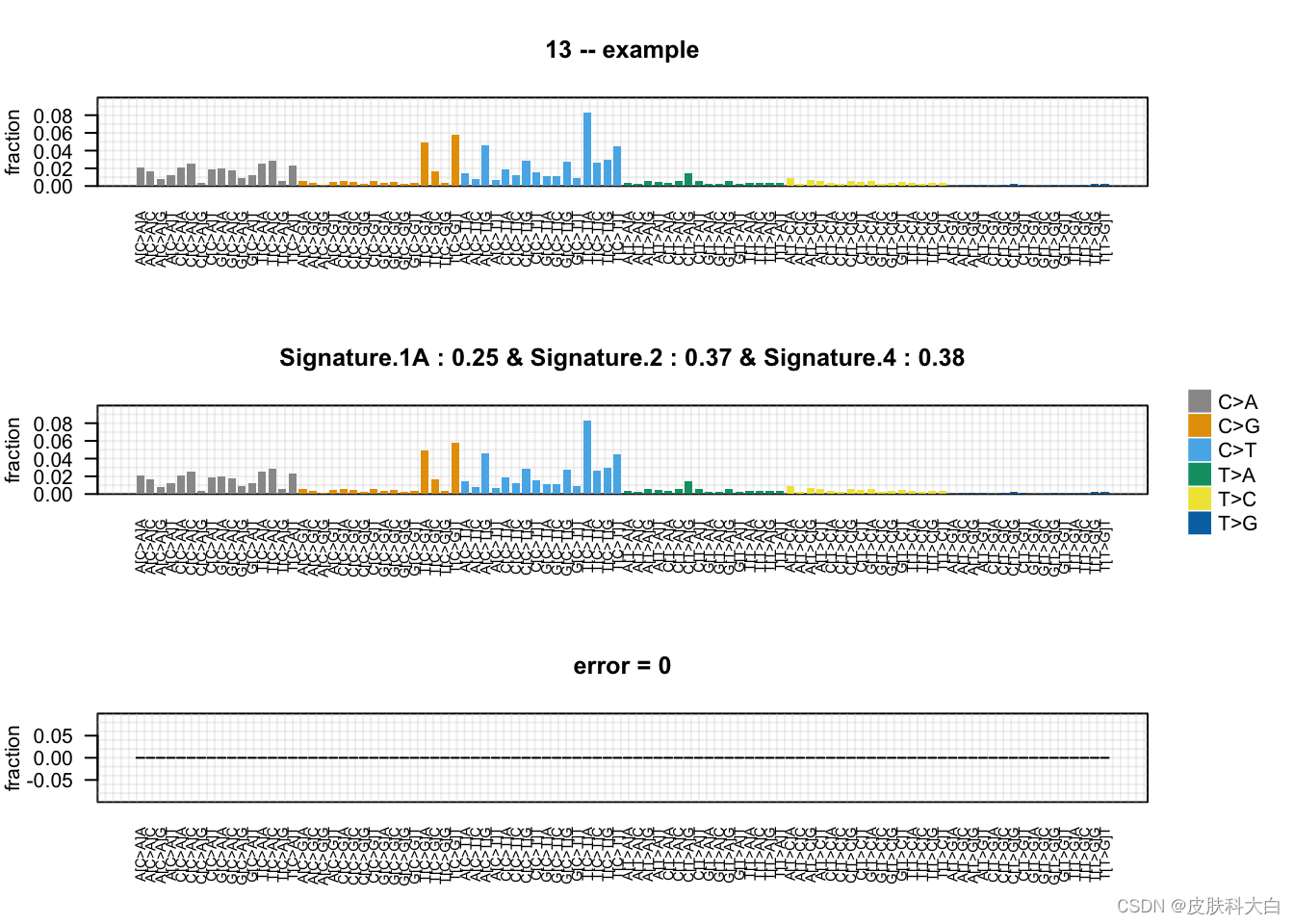
这里是挑出第13个样本,看看它的signature的组成。randomly.generated.tumors是随机生成的一个signature,里面有100个样本,不过要记住,这个数据集里面的样本,其实是一堆样本的意思。因为对单个样本算signature意义不大,单个样本,如果是WES,那么somatic mutation可能就百来个而已。