Deep Neural Network for Image Classification: Application
深度神经网络应用
When you finish this, you will have finished the last programming assignment of Week 4, and also the last programming assignment of this course!
You will use use the functions you’d implemented in the previous assignment to build a deep network, and apply it to cat vs non-cat classification. Hopefully, you will see an improvement in accuracy relative to your previous logistic regression implementation.
After this assignment you will be able to:
- Build and apply a deep neural network to supervised learning.
Let’s get started!
1 - Packages
Let’s first import all the packages that you will need during this assignment.
- numpy is the fundamental package for scientific computing with Python.
- matplotlib is a library to plot graphs in Python.
- h5py is a common package to interact with a dataset that is stored on an H5 file.
- PIL and scipy are used here to test your model with your own picture at the end.
- dnn_app_utils provides the functions implemented in the “Building your Deep Neural Network: Step by Step” assignment to this notebook.
- np.random.seed(1) is used to keep all the random function calls consistent. It will help us grade your work.
导入程序使用的包和模块:
import time
import numpy as np
import h5py
import matplotlib.pyplot as plt
import scipy
from PIL import Image
from scipy import ndimage
from dnn_app_utils_v2 import *

%matplotlib inline
plt.rcParams['figure.figsize'] = (5.0, 4.0) # set default size of plots
plt.rcParams['image.interpolation'] = 'nearest'
plt.rcParams['image.cmap'] = 'gray'

%load_ext autoreload
%autoreload 2

np.random.seed(1)
2 - Dataset
You will use the same “Cat vs non-Cat” dataset as in “Logistic Regression as a Neural Network” (Assignment 2). The model you had built had 70% test accuracy on classifying cats vs non-cats images. Hopefully, your new model will perform a better!
Problem Statement: You are given a dataset (“data.h5”) containing:
- a training set of m_train images labelled as cat (1) or non-cat (0)
- a test set of m_test images labelled as cat and non-cat
- each image is of shape (num_px, num_px, 3) where 3 is for the 3 channels (RGB).
Let’s get more familiar with the dataset. Load the data by running the cell below.
train_x_orig, train_y, test_x_orig, test_y, classes = load_data()
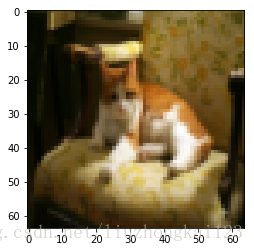
The following code will show you an image in the dataset. Feel free to change the index and re-run the cell multiple times to see other images.
显示一张图片:
index = 7
plt.imshow(train_x_orig[index])#要求输入64*64*3的数组
print ("y = " + str(train_y[0,index]) + ". It's a " + classes[train_y[0,index]].decode("utf-8") +  " picture.")
结果:
y = 1. It's a cat picture.
得到训练样本数、图片分辨率、测试数据样本数的值:
m_train = train_x_orig.shape[0]
num_px = train_x_orig.shape[1]
m_test = test_x_orig.shape[0]

print ("Number of training examples: " + str(m_train))
print ("Number of testing examples: " + str(m_test))
print ("Each image is of size: (" + str(num_px) + ", " + str(num_px) + ", 3)")
print ("train_x_orig shape: " + str(train_x_orig.shape))
print ("train_y shape: " + str(train_y.shape))
print ("test_x_orig shape: " + str(test_x_orig.shape))
print ("test_y shape: " + str(test_y.shape))
结果,训练集209,测试集50:
Number of training examples: 209
Number of testing examples: 50
Each image is of size: (64, 64, 3)
train_x_orig shape: (209, 64, 64, 3)
train_y shape: (1, 209)
test_x_orig shape: (50, 64, 64, 3)
test_y shape: (1, 50)
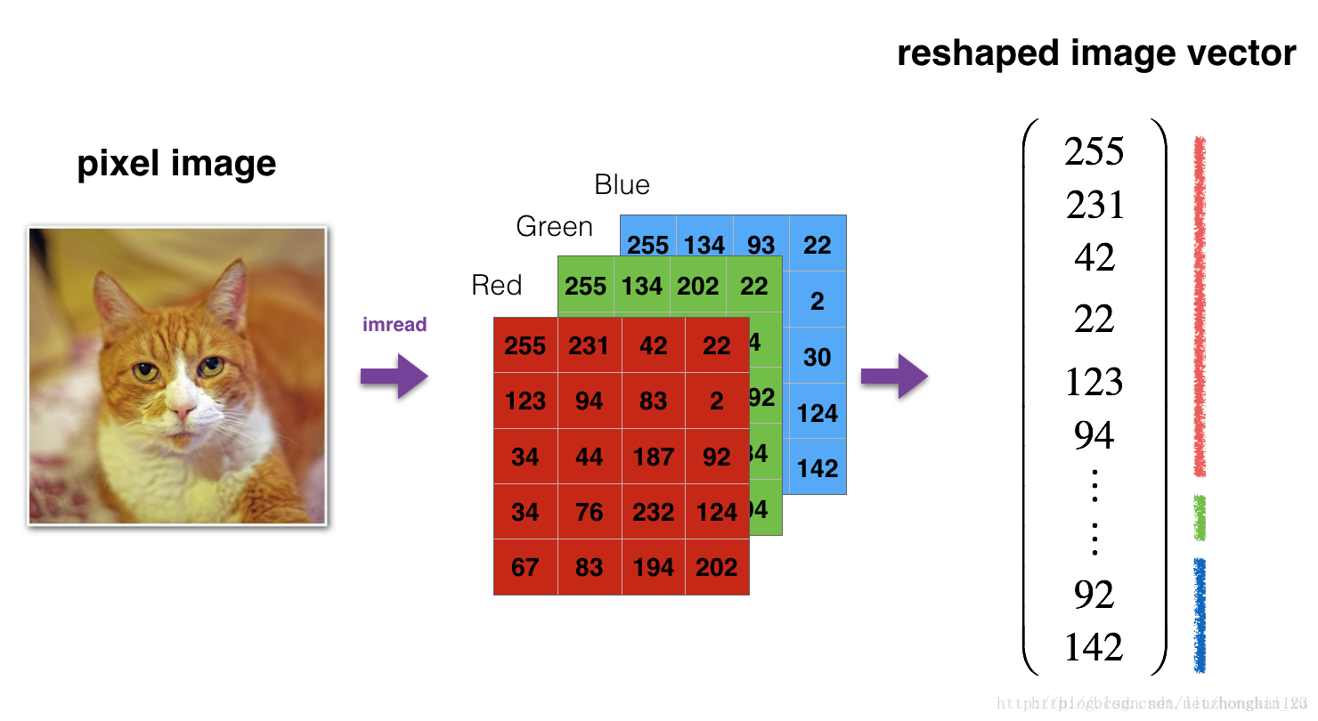
As usual, you reshape and standardize the images before feeding them to the network. The code is given in the cell below. 将图片数组展开为一列。
train_x_flatten=train_x_orig.reshape(train_x_orig.shape[0],-1).T#行209,列根据数组自行展开(12288)
test_x_flatten=test_x_orig.reshape(test_x_orig.shape[0],-1).T
train_x=train_x_flatten/255 #将数组范围限定在0~1
test_x=test_x_flatten/255
print("train_x's shape : ",train_x.shape)
print("test_x's shape : ",test_x.shape)
结果:
train_x's shape :  (12288, 209)
test_x's shape :  (12288, 50)
12,288 equals 64×64×3 which is the size of one reshaped image vector.
3 - Architecture of your model
建立一个两层神经网络和一个多层神经网络
Now that you are familiar with the dataset, it is time to build a deep neural network to distinguish cat images from non-cat images.
You will build two different models:
- A 2-layer neural network
- An L-layer deep neural network
You will then compare the performance of these models, and also try out different values for L.
Let’s look at the two architectures.
3.1 - 2-layer neural network
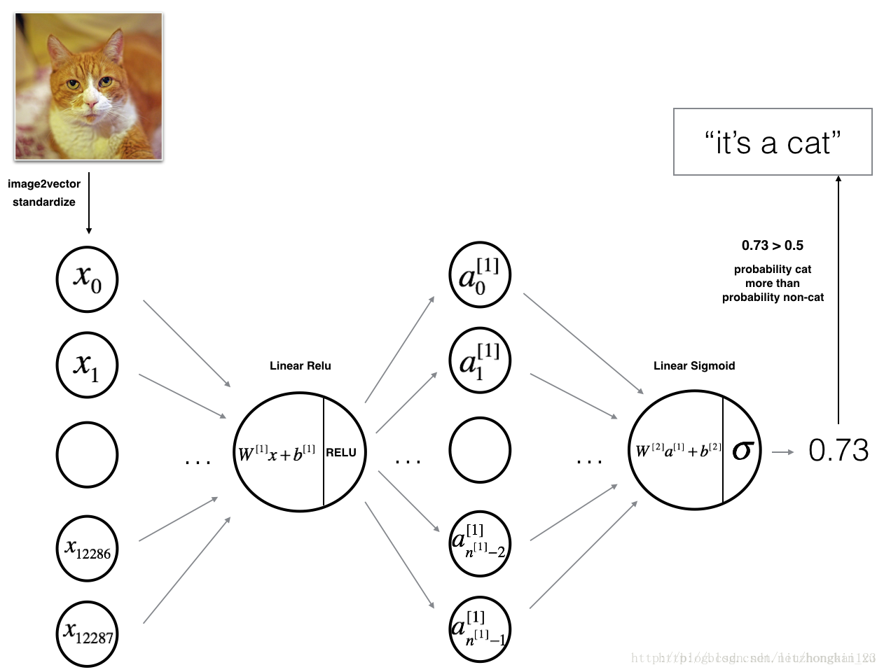
Detailed Architecture of figure 2:
- The input is a (64,64,3) image which is flattened to a vector of size (12288,1).
- The corresponding vector:
[x0,x1,...,x12287]T
is then multiplied by the weight matrix
W[1]
of size (
n[1]
,12288).
- You then add a bias term and take its relu to get the following vector:
[a[1]0,a[1]1,...,a[1]n[1]−1]T
.
- You then repeat the same process.
- You multiply the resulting vector by
W[2]
and add your intercept (bias).
- Finally, you take the sigmoid of the result. If it is greater than 0.5, you classify it to be a cat.
3.2 - L-layer deep neural network
It is hard to represent an L-layer deep neural network with the above representation. However, here is a simplified network representation:
Detailed Architecture of figure 3:
- The input is a (64,64,3) image which is flattened to a vector of size (12288,1).
- The corresponding vector:
[x0,x1,...,x12287]T
is then multiplied by the weight matrix
W[1]
and then you add the intercept
b[1]
. The result is called the linear unit.
- Next, you take the relu of the linear unit. This process could be repeated several times for each (
W[1]
,
b[1]
) depending on the model architecture.
- Finally, you take the sigmoid of the final linear unit. If it is greater than 0.5, you classify it to be a cat.
3.3 - General methodology
As usual you will follow the Deep Learning methodology to build the model:
1. Initialize parameters / Define hyperparameters
2. Loop for num_iterations:
a. Forward propagation
b. Compute cost function
c. Backward propagation
d. Update parameters (using parameters, and grads from backprop)
4. Use trained parameters to predict labels
Let’s now implement those two models!
4 - Two-layer neural network
Question: Use the helper functions you have implemented in the previous assignment to build a 2-layer neural network with the following structure: LINEAR -> RELU -> LINEAR -> SIGMOID. The functions you may need and their inputs are:
### CONSTANTS DEFINING THE MODEL ####
n_x = 12288     # num_px * num_px * 3
n_h = 7
n_y = 1
layers_dims = (n_x, n_h, n_y)
两层神经网咯模型函数
def two_layer_model(X,Y,layers_dims,learning_rate=0.0075,num_iterations=3000,print_cost=True):
np.random.seed(1)
grads = {}
costs = [] # to keep track of the cost
m = X.shape[1] # number of examples
(n_x, n_h, n_y) = layers_dims
#m=X.shape[1]
#n_x,n_h,n_y=layer_dims
parameters=initialize_parameters(n_x,n_h,n_y)
W1 = parameters["W1"]
b1 = parameters["b1"]
W2 = parameters["W2"]
b2 = parameters["b2"]
#Z,cache=linear_forward(A,W,b)
for i in range(0,num_iterations):
A1, cache1=linear_activation_forward(X,W1,b1,'relu')
A2, cache2=linear_activation_forward(A1,W2,b2,'sigmoid')
cost=compute_cost(A2, Y)
dA2=-(np.divide(Y,A2)-np.divide(1-Y,1-A2))
dA1, dW2, db2=linear_activation_backward(dA2,cache2,'sigmoid')
dA0, dW1, db1=linear_activation_backward(dA1,cache1,'relu')
grads['dW1'] = dW1
grads['db1'] = db1
grads['dW2'] = dW2
grads['db2'] = db2
parameters = update_parameters(parameters, grads, learning_rate)
W1 = parameters["W1"]
b1 = parameters["b1"]
W2 = parameters["W2"]
b2 = parameters["b2"]
if print_cost and i % 100 == 0:
print("Cost after iteration {}: {}".format(i, np.squeeze(cost)))
if print_cost and i % 100 == 0:
costs.append(cost)
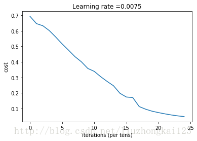
plt.plot(np.squeeze(costs))
plt.ylabel('cost')
plt.xlabel('iterations (per tens)')
plt.title("Learning rate =" + str(learning_rate))
plt.show()
return parameters
测试:
parameters = two_layer_model(train_x, train_y, layers_dims = (n_x, n_h, n_y), num_iterations = 2500, print_cost=True)
结果:
Cost after iteration 0: 0.693049735659989
Cost after iteration 100: 0.6464320953428849
Cost after iteration 200: 0.6325140647912677
Cost after iteration 300: 0.6015024920354665
Cost after iteration 400: 0.5601966311605747
Cost after iteration 500: 0.5158304772764729
Cost after iteration 600: 0.47549013139433266
Cost after iteration 700: 0.4339163151225749
Cost after iteration 800: 0.40079775362038844
Cost after iteration 900: 0.3580705011323798
Cost after iteration 1000: 0.3394281538366413
Cost after iteration 1100: 0.30527536361962654
Cost after iteration 1200: 0.2749137728213016
Cost after iteration 1300: 0.2468176821061486
Cost after iteration 1400: 0.19850735037466108
Cost after iteration 1500: 0.17448318112556668
Cost after iteration 1600: 0.17080762978097128
Cost after iteration 1700: 0.11306524562164709
Cost after iteration 1800: 0.09629426845937152
Cost after iteration 1900: 0.0834261795972687
Cost after iteration 2000: 0.07439078704319084
Cost after iteration 2100: 0.06630748132267933
Cost after iteration 2200: 0.059193295010381744
Cost after iteration 2300: 0.053361403485605606
Cost after iteration 2400: 0.04855478562877022
迭代次数增加cost减小,收敛
predictions_train = predict(train_x, train_y, parameters)
Accuracy: 1.0
predictions_test = predict(test_x, test_y, parameters)
Accuracy: 0.72
存在过拟合问题
Note: You may notice that running the model on fewer iterations (say 1500) gives better accuracy on the test set. This is called “early stopping” and we will talk about it in the next course. Early stopping is a way to prevent overfitting.
精度72%,使用测试集测试精度
Congratulations! It seems that your 2-layer neural network has better performance (72%) than the logistic regression implementation (70%, assignment week 2). Let’s see if you can do even better with an L-layer model.
5 - L-layer Neural Network
多层神经网络模型
Question: Use the helper functions you have implemented previously to build an L-layer neural network with the following structure: [LINEAR -> RELU]×(L-1) -> LINEAR -> SIGMOID. The functions you may need and their inputs are:
### CONSTANTS ###
layers_dims = [12288, 20, 7, 5, 1] #  5-layer model
def L_layer_model(X, Y, layers_dims, learning_rate = 0.0075, num_iterations = 3000, print_cost=False):#lr was 0.009
"""
Implements a L-layer neural network: [LINEAR->RELU]*(L-1)->LINEAR->SIGMOID.
Arguments:
X -- data, numpy array of shape (number of examples, num_px * num_px * 3)
Y -- true "label" vector (containing 0 if cat, 1 if non-cat), of shape (1, number of examples)
layers_dims -- list containing the input size and each layer size, of length (number of layers + 1).
learning_rate -- learning rate of the gradient descent update rule
num_iterations -- number of iterations of the optimization loop
print_cost -- if True, it prints the cost every 100 steps
Returns:
parameters -- parameters learnt by the model. They can then be used to predict.
"""
np.random.seed(1)
costs = [] # keep track of cost
# Parameters initialization.
### START CODE HERE ###
parameters = initialize_parameters_deep(layers_dims)
### END CODE HERE ###
# Loop (gradient descent)
for i in range(0, num_iterations):
# Forward propagation: [LINEAR -> RELU]*(L-1) -> LINEAR -> SIGMOID.
### START CODE HERE ### (≈ 1 line of code)
AL, caches = L_model_forward(X, parameters)
### END CODE HERE ###
# Compute cost.
### START CODE HERE ### (≈ 1 line of code)
cost = compute_cost(AL, Y)
### END CODE HERE ###
# Backward propagation.
### START CODE HERE ### (≈ 1 line of code)
grads = L_model_backward(AL, Y, caches)
### END CODE HERE ###
# Update parameters.
### START CODE HERE ### (≈ 1 line of code)
parameters = update_parameters(parameters, grads, learning_rate)
### END CODE HERE ###
# Print the cost every 100 training example
if print_cost and i % 100 == 0:
print ("Cost after iteration %i: %f" %(i, cost))
if print_cost and i % 100 == 0:
costs.append(cost)
# plot the cost
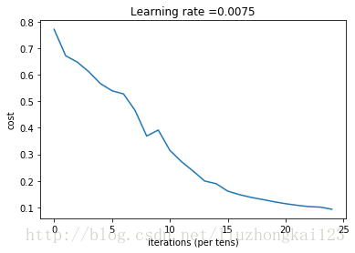
plt.plot(np.squeeze(costs))
plt.ylabel('cost')
plt.xlabel('iterations (per tens)')
plt.title("Learning rate =" + str(learning_rate))
plt.show()
return parameters
You will now train the model as a 5-layer neural network.
Run the cell below to train your model. The cost should decrease on every iteration. It may take up to 5 minutes to run 2500 iterations. Check if the “Cost after iteration 0” matches the expected output below, if not click on the square (⬛) on the upper bar of the notebook to stop the cell and try to find your error.
测试:
parameters = L_layer_model(train_x, train_y, layers_dims, num_iterations = 2500, print_cost = True
结果:
Cost after iteration 0: 0.771749
Cost after iteration 100: 0.672053
Cost after iteration 200: 0.648263
Cost after iteration 300: 0.611507
Cost after iteration 400: 0.567047
Cost after iteration 500: 0.540138
Cost after iteration 600: 0.527930
Cost after iteration 700: 0.465477
Cost after iteration 800: 0.369126
Cost after iteration 900: 0.391747
Cost after iteration 1000: 0.315187
Cost after iteration 1100: 0.272700
Cost after iteration 1200: 0.237419
Cost after iteration 1300: 0.199601
Cost after iteration 1400: 0.189263
Cost after iteration 1500: 0.161189
Cost after iteration 1600: 0.148214
Cost after iteration 1700: 0.137775
Cost after iteration 1800: 0.129740
Cost after iteration 1900: 0.121225
Cost after iteration 2000: 0.113821
Cost after iteration 2100: 0.107839
Cost after iteration 2200: 0.102855
Cost after iteration 2300: 0.100897
Cost after iteration 2400: 0.092878
测试:
pred_train = predict(train_x, train_y, parameters)
pred_test = predict(test_x, test_y, parameters)
结果:
Accuracy: 0.985645933014
Accuracy: 0.8
精度提高到80%
Congrats! It seems that your 5-layer neural network has better performance (80%) than your 2-layer neural network (72%) on the same test set.
This is good performance for this task. Nice job!
Though in the next course on “Improving deep neural networks” you will learn how to obtain even higher accuracy by systematically searching for better hyperparameters (learning_rate, layers_dims, num_iterations, and others you’ll also learn in the next course).
6 Results Analysis
First, let’s take a look at some images the L-layer model labeled incorrectly. This will show a few mislabeled images.
总结不能够识别图片特征
print_mislabeled_images(classes, test_x, test_y, pred_test)
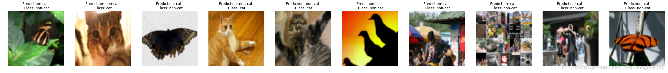
A few type of images the model tends to do poorly on include:
- Cat body in an unusual position
- Cat appears against a background of a similar color
- Unusual cat color and species
- Camera Angle
- Brightness of the picture
- Scale variation (cat is very large or small in image)
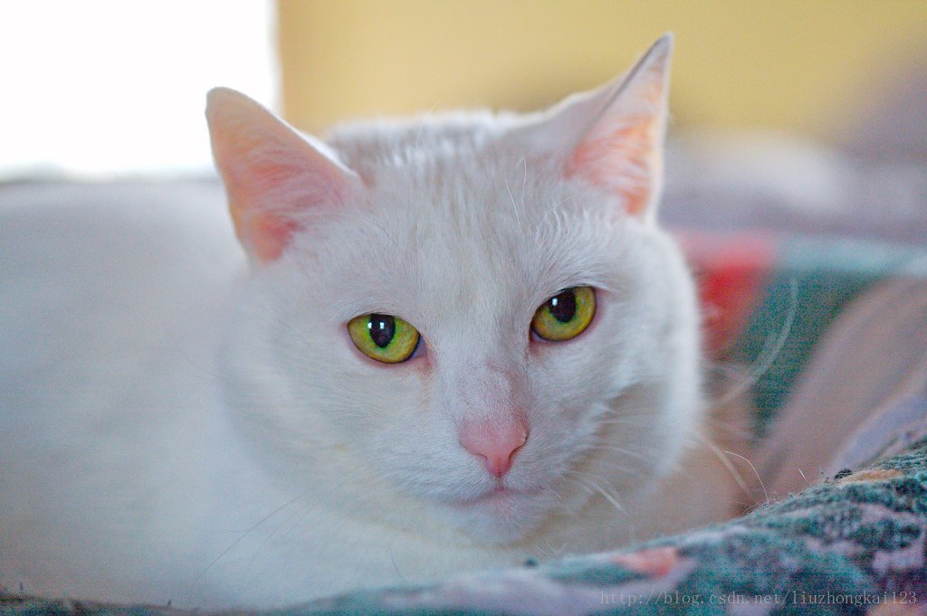
7 Test with your own image (optional/ungraded exercise)
测试自己的图片
Congratulations on finishing this assignment. You can use your own image and see the output of your model. To do that:
1. Click on “File” in the upper bar of this notebook, then click “Open” to go on your Coursera Hub.
2. Add your image to this Jupyter Notebook’s directory, in the “images” folder
3. Change your image’s name in the following code
4. Run the code and check if the algorithm is right (1 = cat, 0 = non-cat)!
## START CODE HERE ##
my_image = "my_image2.jpg" # change this to the name of your image file
my_label_y = [1] # the true class of your image (1 -> cat, 0 -> non-cat)
## END CODE HERE ##

fname = "images/" + my_image
image = np.array(ndimage.imread(fname, flatten=False))
my_image = scipy.misc.imresize(image, size=(num_px,num_px)).reshape((num_px*num_px*3,1))
my_predicted_image = predict(my_image, my_label_y, parameters)

plt.imshow(image)
print ("y = " + str(np.squeeze(my_predicted_image)) + ", your L-layer model predicts a \"" + classes[int(np.squeeze(my_predicted_image)),].decode("utf-8") +  "\" picture.")
Accuracy: 1.0
y = 1.0, your L-layer model predicts a "cat" picture.
References:
for auto-reloading external module: http://stackoverflow.com/questions/1907993/autoreload-of-modules-in-ipython