在这里转载只是为了让不能够科学搜索的同学们看到好文章而已,个人无收益只是分享知识(顺手做个记录罢了)
原网址:https://towardsdatascience.com/over-smoothing-issue-in-graph-neural-network-bddc8fbc2472
Over-smoothing issue in graph neural network
TLDR: This story gives a high-level entry to graph neural network: the How and the Why, before introducing a serious issue that accompanies the message passing framework which represents the main feature of today’s GNN. Don’t forget to use the references below to deepen your understanding of GNNs!
An illustrated guide to Graph neural networks
Graph neural network or GNN for short is deep learning (DL) model that is used for graph data. They have become quite hot these last years. Such a trend is not new in the DL field: each year we see the stand out of a new model, that either shows state-of-the-art results on benchmarks or, a brand new mechanism/framework (but very intuitive when you read about it) into already used models. This reflection makes us question the reason of existence for this new model dedicated to graph data.
Why do we need GNNs?
Graphs are everywhere: Graph data is abundant, and I believe it is the most natural and flexible way to present the material that we generate or consume every day. We needn’t think hard to enumerate a panoply of graph data examples, from relational databases used in most corporations and social networks like Facebook or Twitter, to citation graphs that links knowledge creation in science and literature. Even images could be seen as graphs because of their grid structure.
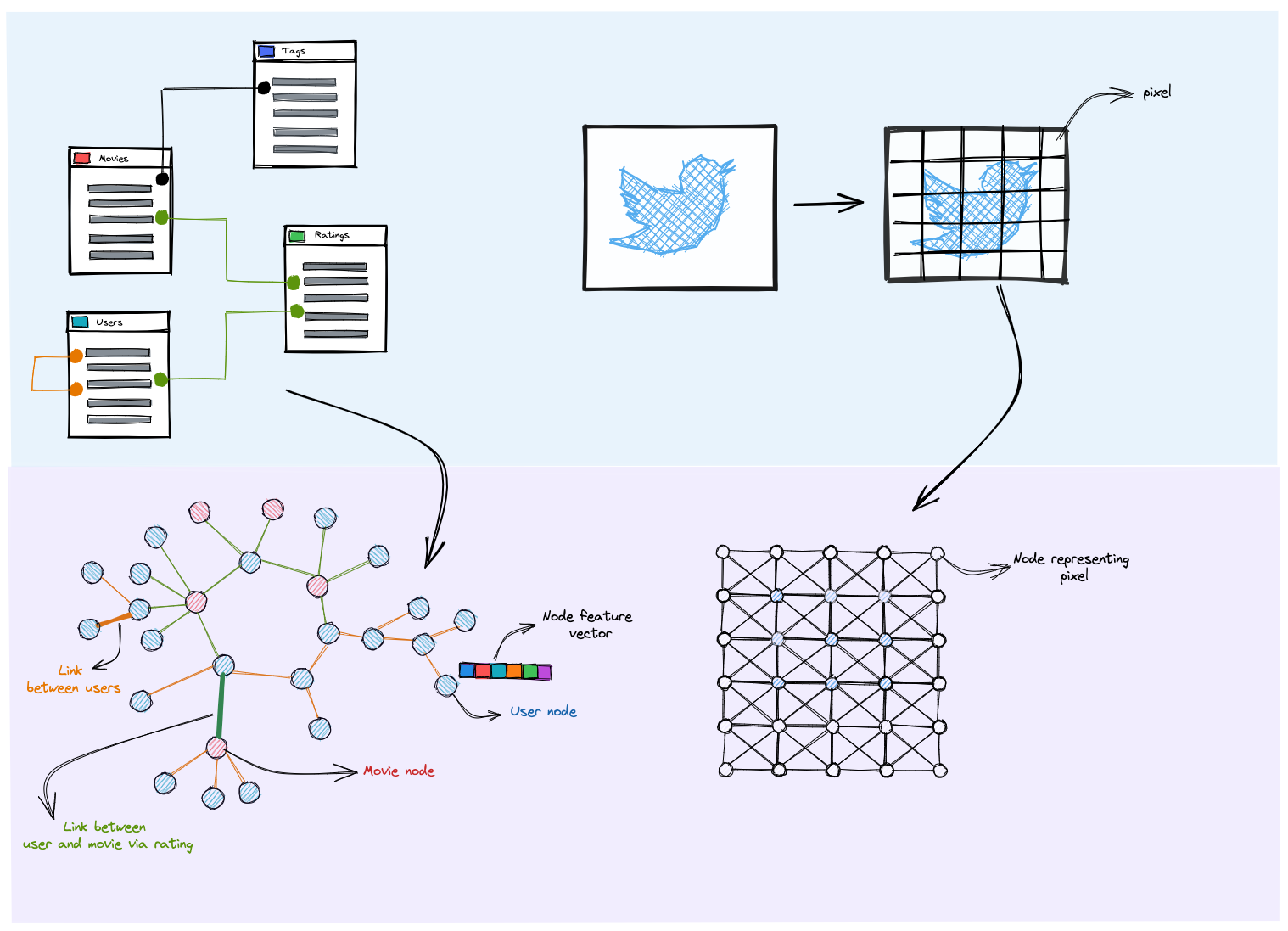
For a relational database, entities are nodes and the relationships (one-to-one, one-to-many ) define our edges. As for images, the pixel are nodes, and neighboring pixels can be used to define edges
Models able to capture all the possible information in graphs: as we saw, graph data is everywhere and takes the form of interconnected nodes with feature vectors. And Yes, we can use some Multilayer Perceptron models to resolve our downstream tasks, but we will be losing the connections that the graph topology offers us. As for convolution neural networks, their mechanisms are dedicated to a special case of graph: grid-structured inputs, where nodes are fully connected with no sparsity. That being said, the only remaining solution is a model that can build upon the information given in both: the nodes’ features and the local structures in our graph, which can ease our downstream task; and that is literally what GNN does.
What tasks do GNNs train on?
Now that we have modestly justified the existence of such models, we shall uncover their usage. In fact, there are a lot of tasks that we can train GNNs on: node classification in large graphs (segment users in a social network based on their attributes and their relations), or whole graph classification (classifying protein structures for pharmaceutical applications). In addition to classification, regression problems can also be formulated on top of graph data, working not only on nodes but on edges as well.
To sum up, graph neural network applications are endless and depend on the user's objective and the type of data that they possess. For the sake of simplicity, we will focus on the node classification task within a unique graph, where we try to map a subset of nodes graph headed by their feature vectors to a set of predefined categories/classes.
The problem supposes the existence of a training set where we have a labeled set of nodes, and that all nodes in our graph got a certain features vector that we note x. Our goal is to predict labels of featured nodes in a validation set.
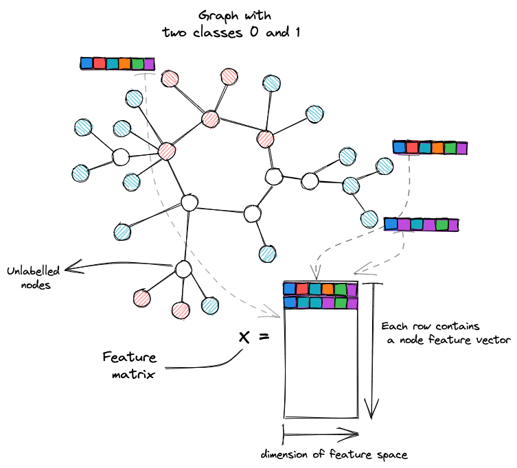
Node classification example: all nodes have a feature vector; colored nodes are labeled, while those in white are unlabeled
GNN under the hood
Now that we have set our problem, it's time to understand how the GNN model will be trained to output classes for unlabelled nodes. In fact, we want our model not only to use the feature vectors of our nodes but also to take advantage of the graph structure of which we dispose of.
This last statement, which makes the GNN unique, must be boxed within a certain hypothesis which states that neighbor nodes tend to share the same label. GNN incorporates that by using message passing formalism, a concept that will be discussed further in this article. We will introduce some of the bottlenecks that we will consider posteriorly.
Enough abstraction, let us now look at how are GNNs constructed. In fact, a GNN model contains a series of layers that communicate via an updated node representation (each layer outputs an embedding vector for each node, which is then used as an input for the next layer to build upon it).
The purpose of our model is to construct these embeddings (for each node) integrating both the nodes' initial feature vector and the information about the local graph structure that surrounds them. Once we have well-representing embeddings, we feed a classical Softmax layer to those embeddings to output relative classes.
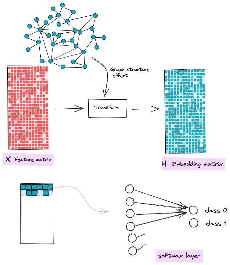
The goal of GNN is to transform node features to features that are aware of the graph structure
To build those embeddings, GNN layers use a straightforward mechanism called message passing, which helps graph nodes exchange information with their neighbors, and thus update their embedding vector layer after layer.
- The message passing framework
It all starts with some nodes with vector x describing their attributes, then each node collects other feature vectors from its neighbors’ nodes via a permutation equivariant function (mean, max, min ..). In other words, a function that is not sensible to nodes ordering. This operation is called Aggregate, and it outputs a Message vector.
The second step is the Update function, where the node combines the information gathered from its neighbors (Message vector) with its own information (its feature vector ) to construct a new vector h: Embedding.
The instantiation of this aggregate and update functions differ from one paper to another. You can refer to GCN[1], GraphSage[2], GAT[3], or others, but the message passing idea stays the same.
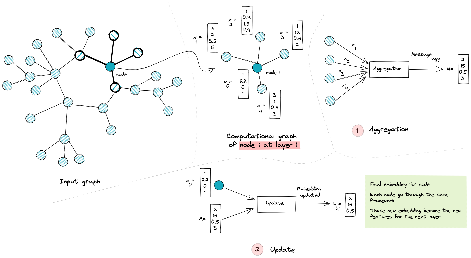
an illustration of the first layer of our GNN model from feature vector x0 to its new embedding h
What is the intuition behind this framework? Well, we want our node’s new embedding to make allowances for the local graph structure, that is why we aggregate information from neighbors’ nodes. By doing so, one could intuitively foresee that a set of neighbor nodes after aggregating will have a more similar representation, which will ease our classification task at the end. All that in the case where our first hypothesis (neighbor nodes tend to share the same label) always stands.
- Layers composition in GNNs
Now that we have understood the main mechanism of message passing, it's time to understand what layers mean in the context of GNN.
Recall to the last section, each node uses the information from its neighbors to update its embeddings, thus a natural extension is to use the information from the neighbors of its neighbors(or second-hop neighbors ) to increase its receptive field and become more aware of the graph structure. This is what makes the second layer of our GNN model.
We can generalize this to N layers by aggregating information from N hop neighbors.
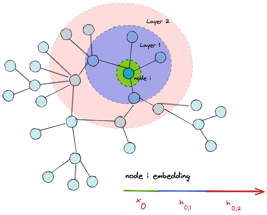
Layer after layer, nodes have access to more graph nodes and a more graph structure-aware embedding
At this point, You have a high-level understanding of how GNNs work, and you may be able to detect why there will be issues with this formalism. First of all, talking about GNN in the context of deep learning supposes the existence of depth (many layers). This means nodes will have access to information from nodes that are far and may not be similar to them. On one hand, the message passing formalism tries to soften out the distance between neighbors nodes (smoothing ) to ease our classification later. On the other hand, it can work in the other direction by making all our nodes embedding similar thus we will not be able to classify unlabeled nodes (over-smoothing ).
In the next section, I will try to explain what is smoothing and over-smoothing, we discuss smoothing as a natural effect of increasing GNN layers, and we will see why it can be an issue.
I will also try to quantify it (thus making it trackable) and build upon this quantification to resolve it using solutions from published papers on this issue.
Over-smoothing issue in GNNs
Although the message passing mechanism helps us harness the information encapsulated in the graph structure, it may introduce some limitations if combined with GNN depth. In other words, our quest for a model that is more expressive and aware of the graph structure (by adding more layers so that nodes can have a large receptive field) could be transformed into a model that treats nodes all the same (the node representations converging to indistinguishable vectors[4]).
This smoothing phenomenon is not a bug nor a special case, but an essential nature for GNN, and our goal is to alleviate it.
Why does over-smoothing happen?
The message passing framework uses the two main functions introduced earlier Aggregate and Update, which gather feature vectors from neighbors and combine them with the nodes’ own features to update their representation. This operation works in a way that makes interacting nodes (within this process) have quite similar representations.
We will try to illustrate this in the first layer of our model to show why smoothing happens, then add more layers to show how this representation smoothing increases with layers.
Note : The over-smoothing shows itself in the form of similarity between nodes’ embedding. So we use colors, where different colors mean a difference in the vector embeddings . Moreover, for the sake of simplicity in our example, we will only update the 4 nodes highlighted .
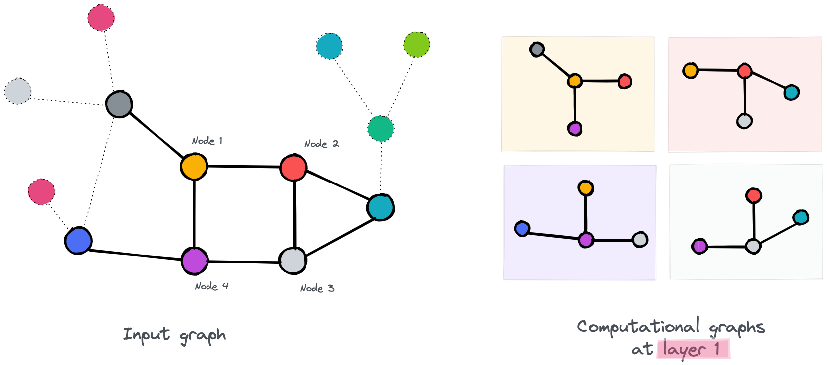
the first layer of our GNN
As you can see in the first layer, nodes have access to one-hop neighbors. You may also observe, for example, that node 2 and node 3 have almost access to the same information since they are linked to each other and have common neighbors, and that the only difference is in their last neighbor(purple and yellow). We can predict that their embeddings will be slightly similar. As for Node 1 and Node 4, they interact with each other but have different neighbors. So we may predict that their new embeddings will be different.
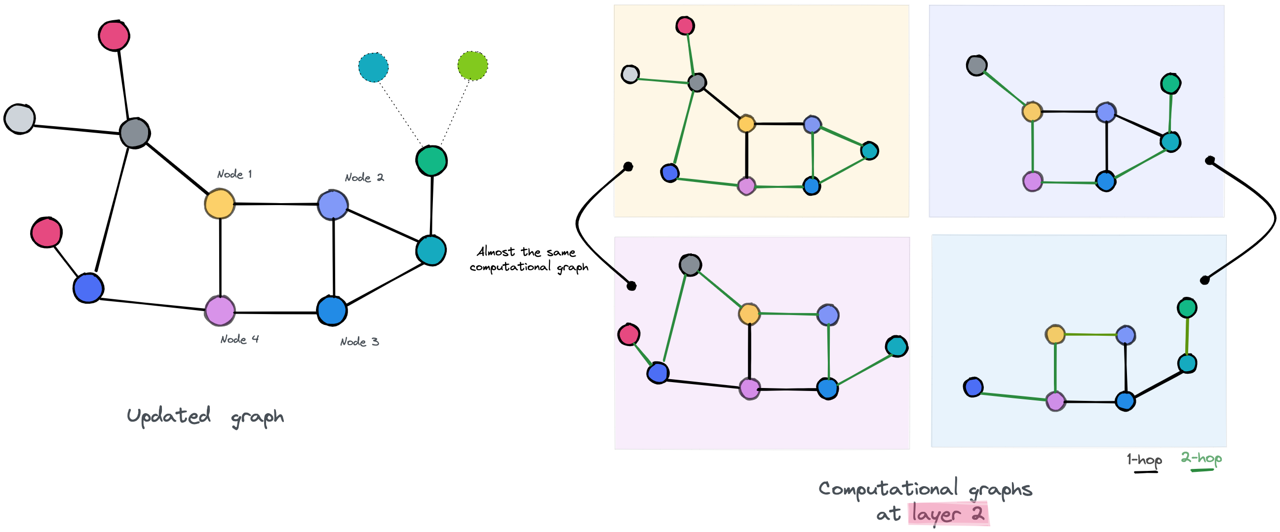
We update our graph by assigning to each node its new embedding and move to the second layer and do over the same process.
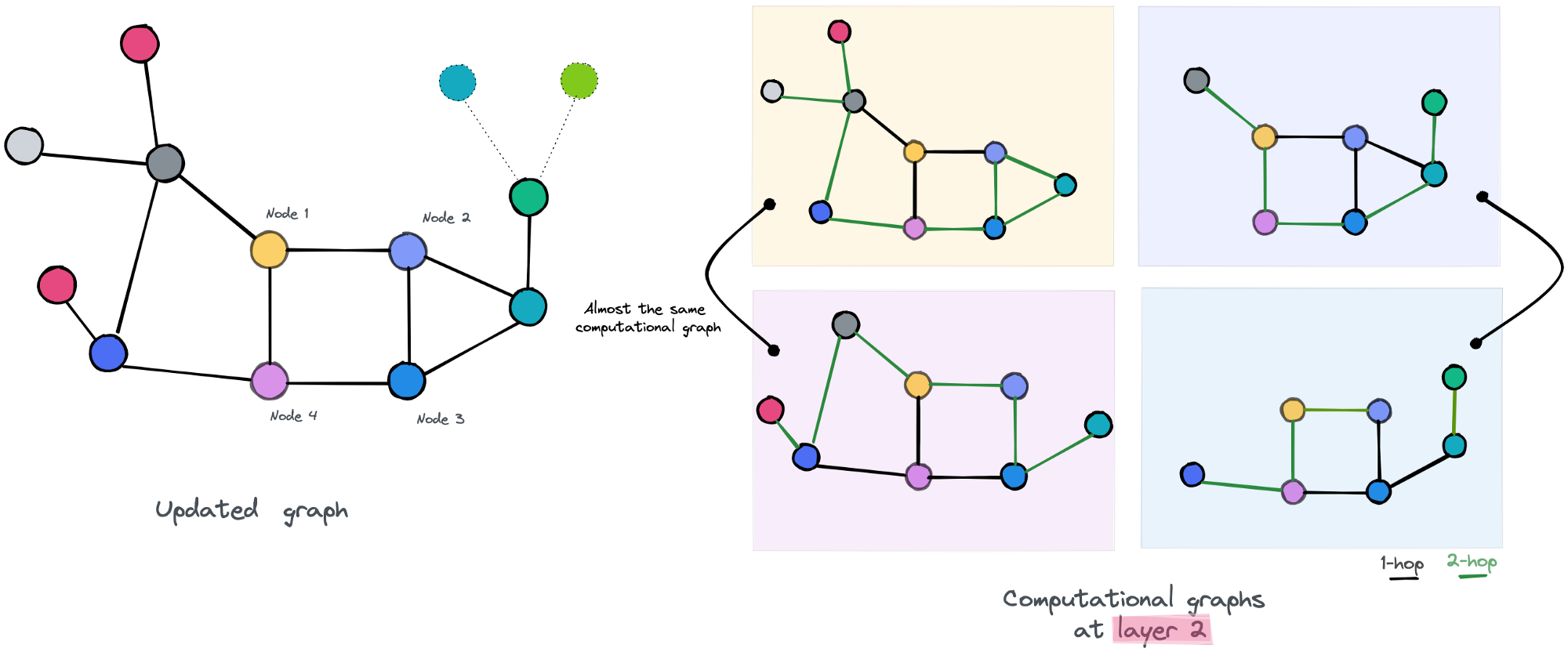
the second layer of our GNN
It the second layer of our GNN, the computational graphs of nodes 1,4, and 2,3 are almost the same respectively. We may expect that our new updated embedding for those nodes will be more similar, even for the node 1 and node 4 that “survived” in a way the first layer, will now have similar embeddings, since the extra layer gives them access to more of the graph’s parts, increasing the probability of accessing to the same nodes.
This simplified example shows how over-smoothing is a result of depth in GNN. It's fair to say it’s far from real cases, but it still gives an idea of the reason behind the occurrence of this phenomenon.
Why is it really an issue?
Now that we understand why over-smoothing happens, and why it is by design, an effect of GNN layer composition, it's time to emphasize why we should care about it, and motivate solutions to overcome it.
First things first, the goal from learning our embeddings is to feed them to a classifier at the end, in order to predict their labels. Having this over-smoothing effect in mind, we will end up with similar embeddings for nodes that don't have the same label, which will result in mislabeling them.
One may think that reducing the number of layers will reduce the effect of over-smoothing. Yes, but this implies not exploiting the multi-hop information in the case of complex-structured data, and consequently not boosting our end-task performance.
Example: To emphasis this last statement, I will illustrate it with an example that’s frequent in real-life scenarios. Imagine that we're dealing with a social network graph with thousands of nodes. Some new users just signed in to the platform and subscribed to their friend's profiles. Our goal is to find topic suggestions to fill their feed.
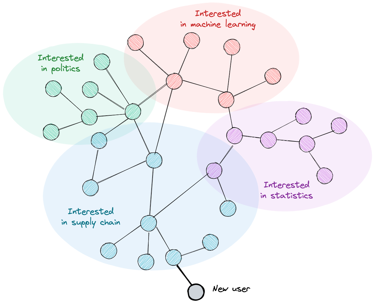
An imaginary social network
Given this imaginary social network, Using only 1 or 2 layers in our GNN model, we will only learn that our user cares about supply chain topics, but we miss other diversified topics that he may like given his friend’s interactions.
To sum up, having over-smoothing as an issue, we encounter a trade-off between a low-efficiency model and a model with more depth but less expressivity in terms of node representations.
How can we quantify it?
Now that we’ve made it clear that over-smoothing is an issue and that we should care about it, we have to quantify it, so that we can track it while training our GNN model. Not only this, but quantifying will also offer us a metric to be used as a numerical penalization by adding it as a regularization term in our objective function (Or not …).
According to my last readings, plenty of papers treated the over smoothing issue in GNN, and they have all proposed a metric to quantify it to prove their hypothesis about the issue and validate their solutions to it.
I selected two metrics from two different papers that treated this issue.
Deli Chen et al introduced two quantitative metrics, MAD and MADGap, to measure the smoothness and over-smoothness of the graph nodes representations.
On one hand, the MAD calculates the Mean Average Distance among node representations (embeddings) in the graph and uses it to show that smoothing is a natural effect of adding more layers to the GNN model. Based on this measure, they extended it to MADGap which measures the similarity of representations among different classes of nodes. This generalization was built on the main hypothesis that while nodes are interacting, they have either access to important information from nodes from the same class or noise by interacting with nodes from other classes.
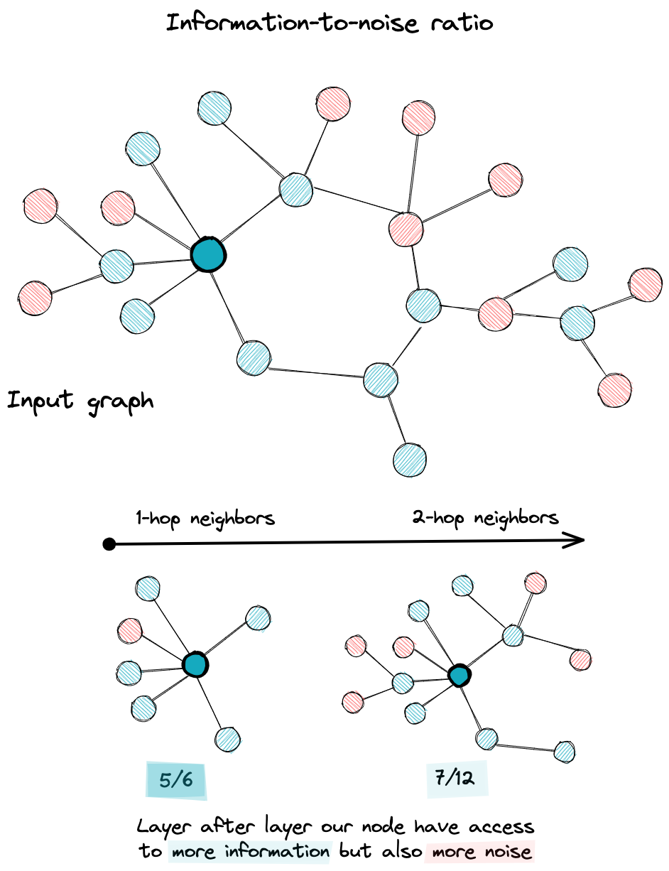
while node access to more parts of the graph we may access to noisy nodes that affect the final embedding
What intrigued me in this paper was the way the authors questioned the main hypothesis upon which the message passing formalism is built (neighbor nodes may have similar labels). In fact, their measure MADGap goes beyond being a measure of over smoothing to be seen as a measure of information-to-noise ratio relative to the signals gathered by our nodes. As a result, observing that this ratio decreases layer after layer is proof of discrepancy between the graph topology and the objective of the downstream task.
Kaixiong Zhou et al introduced another strain forward metric but with the same objective as MADGap which is Group Distance Ratio. This metric computes two average distances then calculates their ratio. We start first by putting nodes in their specific group relative to their label. Then, to construct the nominator of our ratio, we calculate the pairwise distance between every two groups of nodes, then averages over the resulting distances. As for the denominator, we calculate the average distance for each group then we calculate the mean.
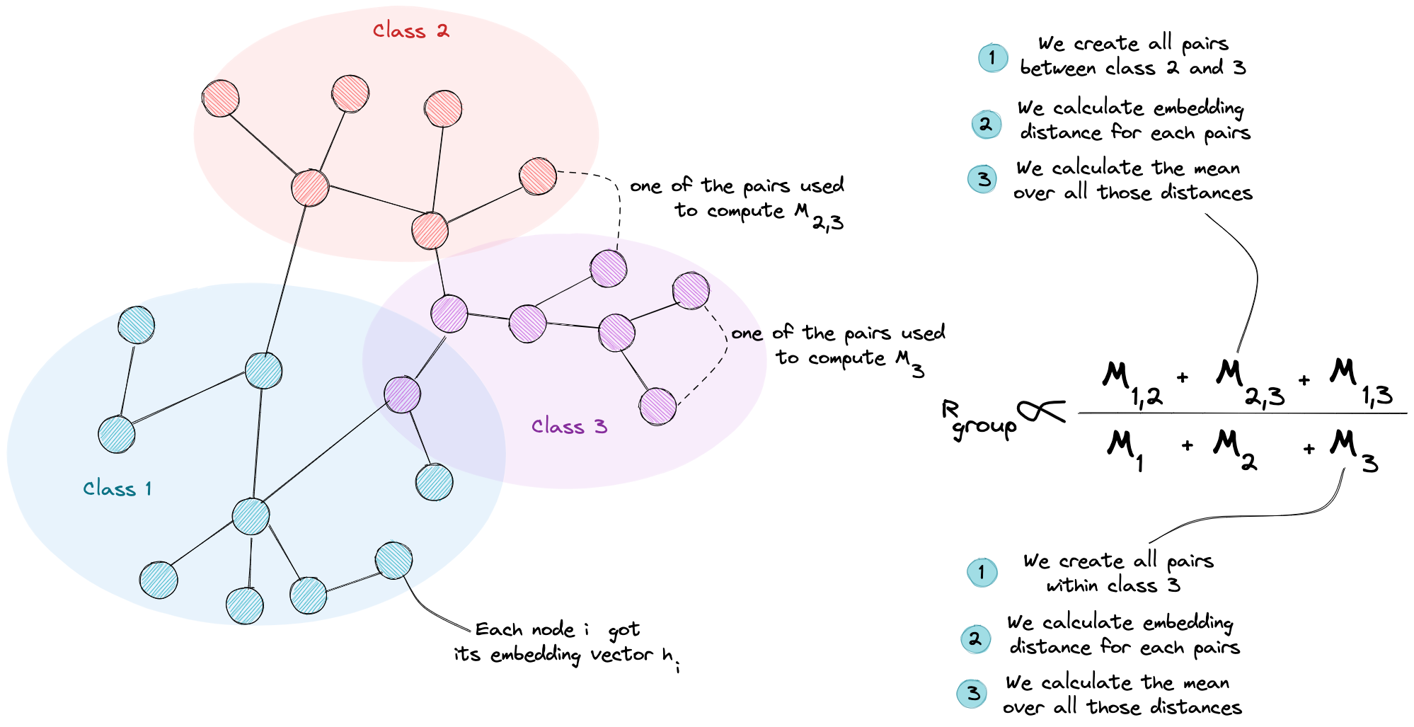
An illustration that explains how the group distance ratio is computed
Having a small ratio means that the average distance between node embedding in different groups is small, thus we may mix groups in terms of their embeddings, which is proof of over-smoothing.
Our goal then is to maintain a high Group Distance Ratio to have a difference between classes of nodes in terms of their embedding which will ease our downstream task.
Are there solutions to overcome over-smoothing?
A direct regulation term?
Now that we have quantified the over smoothing issue, you may think that our job is terminated and that it’s enough to add this metric as a regulation term in our loss objective. The problem remaining is that computing those metrics (mentioned above) at each iteration of our training session could be computationally expensive, since we need access to all training nodes in our graph, and then do some distance calculation that deals with pairs of nodes that scale quadratically (C(2, n) = n * (n -1) / 2 = O(n²)) with the number of nodes.
An indirect solution?
For this reason, all papers discussing the over-smoothing issue thought about overcoming this computing issue by other indirect solutions that are easier to implement and have an effect on over-smoothing. We will not extensively discuss these solutions but you will find the references to some of them below.
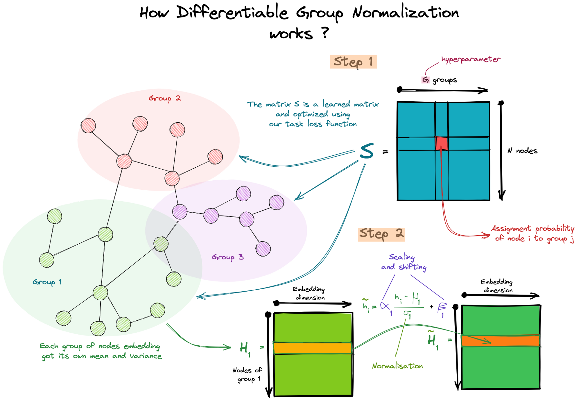
As for our example, we will treat the Differentiable Group Normalization[6] introduced by Kaixiong Zhou et al. DGN assigns nodes into groups and normalizes them independently to output a new embedding matrix for the next layer.
This additional layer is built to optimize the Group Distance Ratio or Rgroup defined previously. In fact, the normalization of nodes embedding within a group makes their embedding quite similar (decreasing the numerator of Rgroup), and these scaling and shifting using the trainable parameters makes the embedding from different groups different (increasing the numerator of Rgroup).
How differentiable group normalization work?
Why does it work? Reading the paper for the first time, I didn't see the connection between adding this normalization layer and the optimization of the Rgrou ratio, then I've observed that this layer uses in one hand a trainable assignment matrix, thus it has feedback from our loss function, so it's guided to assign nodes in the perfect case to their true classes. On the other hand, we have also the shifting and scaling parameters which are also guided by our loss function. Those parameters used to differ embeddings from one group to another thus help in the downstream task.
Opening and conclusions
This article may be long but it only scratches the surface of graph neural networks and their issues, I tried to start by a small exploration of GNNs and show how they can -with such a simple mechanism- unlock potential application that we cannot think of in the context of other DL architecture. this simplicity is constrained with many issues that block their expressiveness (for now …) and the goal of researchers is to overcome it in a quest to harness the full power of graph data.
As for me, I read different papers discussing some of GNNs limits and bottlenecks but the one common point that unifies them is that all of these issues can be linked to the main mechanisms that we use to train our graph models which is Message-passing. I might not be an expert but I must raise some questions about it. Is it really worth it to keep enumerating those issues and trying to fix them? Why not think of a new mechanism and give it a try since we still in the first iteration of such an interesting field?
[1] Kipf, T. N. (2016, September 9). Semi-Supervised Classification with Graph Convolutional Networks. ArXiv.Org. https://arxiv.org/abs/1609.02907
[2] Hamilton, W. L. (2017, June 7). Inductive Representation Learning on Large Graphs. ArXiv.Org. https://arxiv.org/abs/1706.02216
[3] Veličković, P. (2017, October 30). Graph Attention Networks. ArXiv.Org. https://arxiv.org/abs/1710.10903
[4] Oono, K. (2019, May 27). Graph Neural Networks Exponentially Lose Expressive Power for Node Classification. ArXiv.Org. https://arxiv.org/abs/1905.10947
[5] Chen, D. (2019, September 7). Measuring and Relieving the Over-smoothing Problem for Graph Neural Networks from the Topological View. ArXiv.Org. https://arxiv.org/abs/1909.03211
[6] Zhou, K. (2020, June 12). Towards Deeper Graph Neural Networks with Differentiable Group Normalization. ArXiv.Org. https://arxiv.org/abs/2006.06972
I want to express my gratitude to Zineb SAIF and Badr MOUFAD for their contributions to this modest piece. and not to forget my reading team that keep spamming with my draft. Thank you all till we meet in another story