我们今天给大家演示下caret包做随机森林分类的一个小例子,同时也给大家看看做预处理和不做预处理两种情况下的模型表现。
加载R包和数据
rm(list = ls())
library(caret)
## Loading required package: ggplot2
## Loading required package: lattice
load(file = "../000机器学习/hotels_df.rdata")
str(hotels_df)
## tibble [75,166 × 10] (S3: tbl_df/tbl/data.frame)
##  $ children                   : Factor w/ 2 levels "children","none": 2 2 2 2 2 2 2 2 2 2 ...
##  $ hotel                      : Factor w/ 2 levels "City Hotel","Resort Hotel": 2 2 2 2 2 2 2 2 2 2 ...
##  $ arrival_date_month         : Factor w/ 12 levels "April","August",..: 6 6 6 6 6 6 6 6 6 6 ...
##  $ meal                       : Factor w/ 5 levels "BB","FB","HB",..: 1 1 1 1 1 1 1 2 3 1 ...
##  $ adr                        : num [1:75166] 0 0 75 75 98 98 107 103 145 97 ...
##  $ adults                     : num [1:75166] 2 2 1 1 2 2 2 2 2 2 ...
##  $ required_car_parking_spaces: Factor w/ 2 levels "none","parking": 1 1 1 1 1 1 1 1 1 1 ...
##  $ total_of_special_requests  : num [1:75166] 0 0 0 0 1 1 0 1 0 3 ...
##  $ stays_in_week_nights       : num [1:75166] 0 0 1 1 2 2 2 2 4 4 ...
##  $ stays_in_weekend_nights    : num [1:75166] 0 0 0 0 0 0 0 0 0 0 ...
这个数据一共有75166行,10列,数据维度不大,其中children这一列是结果变量,二分类,因子型,其余列都是预测变量。
结果变量两个分类间的差别还是很大的,可以看到大概是10:1的比例:
table(hotels_df$children)
##
## children     none
##     6073    69093
咱们先做一个简单的探索性数据分析看看数据情况,就用咱们之前介绍过很多次的GGally包。
library(ggplot2)
library(GGally)
## Registered S3 method overwritten by 'GGally':
##   method from
##   +.gg   ggplot2

ggbivariate(hotels_df, outcome = "children")+
  scale_fill_brewer(type = "qual")

从这个图可以很清晰的看到结果变量的不平衡,预测变量中有很多是分类变量,几个数值型的预测变量好像在不同类别间的差别不是很大。
不做数据预处理
首先我们演示下不做数据预处理的情况,随机森林是一个“很包容”的算法,它对数据的要求非常低,不做预处理也是可以直接建立模型的。
下面我们直接开始,由于这个数据集不算小,所以运行很慢哈,内存小的电脑可能会直接卡死…
- 划分训练集、测试集,
- 重抽样方法选择10折交叉验证,
- 使用网格搜索,自定义网格范围,
- 在训练集建立模型。
一气呵成:
# 设定种子数
set.seed(3456)

# 根据结果变量的类别多少划分
trainIndex <- createDataPartition(hotels_df$children, p = 0.7,
                                  list = FALSE)
head(trainIndex)
##      Resample1
## [1,]         1
## [2,]         3
## [3,]         5
## [4,]         6
## [5,]         7
## [6,]         9

hotelsTrain <- hotels_df[ trainIndex,]
hotelsTest  <- hotels_df[-trainIndex,]

dim(hotelsTrain)
## [1] 52618    10
dim(hotelsTest)
## [1] 22548    10

# 选择重抽样方法,10折交叉验证
trControl <- trainControl(method = "cv", number = 10,
                          classProbs = T,
                          summaryFunction = twoClassSummary
                          )

# 网格搜索,首先设定超参数范围
rfGrid <-  expand.grid(mtry = seq(2,10,2),
                       splitrule = c( "gini", "extratrees", "hellinger"),
                       min.node.size = seq(1,15,2)
                       )


# 加速,CPU没这么多线程的改小一点
library(doParallel)
## Loading required package: foreach
## Loading required package: iterators
## Loading required package: parallel
cl <- makePSOCKcluster(16)
registerDoParallel(cl)

set.seed(8)

rffit1 <- train(x = hotelsTrain[,-1],
               y = hotelsTrain$children,
               method = "ranger",
               trControl = trControl,
               verbose = FALSE,
               tuneGrid = rfGrid
               )

rffit1
## Random Forest
##
## 52618 samples
##     9 predictor
##     2 classes: 'children', 'none'
##
## No pre-processing
## Resampling: Cross-Validated (10 fold)
## Summary of sample sizes: 47357, 47356, 47356, 47355, 47357, 47356, ...
## Resampling results across tuning parameters:
##
##   mtry  splitrule   min.node.size  ROC        Sens        Spec
##    2    gini         1             0.8768929  0.17827285  0.9952033
##    2    gini         3             0.8767803  0.17944932  0.9953066
##    2    gini         5             0.8761470  0.17685998  0.9955341
##    2    gini         7             0.8764686  0.17450925  0.9955341
##    2    gini         9             0.8759509  0.17451036  0.9956375
##    2    gini        11             0.8759252  0.17286219  0.9958235
##    2    gini        13             0.8759497  0.17004087  0.9958856
##    2    gini        15             0.8754730  0.16886772  0.9958235
##    2    extratrees   1             0.8675842  0.06773488  0.9992970
##    2    extratrees   3             0.8673029  0.06538470  0.9994624
##    2    extratrees   5             0.8672041  0.06373488  0.9995245
##    2    extratrees   7             0.8666000  0.06161944  0.9995451
##    2    extratrees   9             0.8664335  0.06020878  0.9995658
##    2    extratrees  11             0.8660962  0.05997349  0.9995038
##    2    extratrees  13             0.8659157  0.05550511  0.9995245
##    2    extratrees  15             0.8656270  0.05644573  0.9996278
##    2    hellinger    1             0.8785511  0.16275283  0.9962371
##    2    hellinger    3             0.8779519  0.16274896  0.9964025
##    2    hellinger    5             0.8779581  0.16228224  0.9962577
##    2    hellinger    7             0.8773762  0.15851754  0.9962784
##    2    hellinger    9             0.8774350  0.15992985  0.9963818
##    2    hellinger   11             0.8768638  0.15616791  0.9964231
##    2    hellinger   13             0.8769271  0.15334548  0.9965679
##    2    hellinger   15             0.8765844  0.15428445  0.9965059
##    4    gini         1             0.8766326  0.31373985  0.9860233
##    4    gini         3             0.8767241  0.30268600  0.9869950
##    4    gini         5             0.8773796  0.29610329  0.9880909
##    4    gini         7             0.8777288  0.28763325  0.9886491
##    4    gini         9             0.8781637  0.28457664  0.9894555
##    4    gini        11             0.8783674  0.27752168  0.9899103
##    4    gini        13             0.8787160  0.27187849  0.9900757
##    4    gini        15             0.8783649  0.26717371  0.9905099
##    4    extratrees   1             0.8758849  0.24365369  0.9902825
##    4    extratrees   3             0.8761048  0.23542171  0.9909648
##    4    extratrees   5             0.8762743  0.22789616  0.9924948
##    4    extratrees   7             0.8767513  0.21966529  0.9929910
##    4    extratrees   9             0.8767754  0.21425463  0.9934252
##    4    extratrees  11             0.8768805  0.20484618  0.9939627
##    4    extratrees  13             0.8769265  0.20061585  0.9945003
##    4    extratrees  15             0.8768345  0.19497045  0.9947898
##    4    hellinger    1             0.8785093  0.30715327  0.9867056
##    4    hellinger    3             0.8790078  0.30221431  0.9874706
##    4    hellinger    5             0.8793307  0.29868931  0.9881736
##    4    hellinger    7             0.8796394  0.29186854  0.9887732
##    4    hellinger    9             0.8797965  0.28457885  0.9893728
##    4    hellinger   11             0.8802855  0.28010936  0.9897449
##    4    hellinger   13             0.8803949  0.27493344  0.9899310
##    4    hellinger   15             0.8806475  0.27140679  0.9901585
##    6    gini         1             0.8725440  0.33960177  0.9822603
##    6    gini         3             0.8733587  0.33349020  0.9839558
##    6    gini         5             0.8741924  0.32196907  0.9854857
##    6    gini         7             0.8753984  0.31209279  0.9865402
##    6    gini         9             0.8756844  0.30574427  0.9874500
##    6    gini        11             0.8762144  0.30198012  0.9879669
##    6    gini        13             0.8758602  0.29703894  0.9882770
##    6    gini        15             0.8768813  0.28857332  0.9888972
##    6    extratrees   1             0.8712914  0.30057332  0.9835008
##    6    extratrees   3             0.8732889  0.28622535  0.9859819
##    6    extratrees   5             0.8742153  0.27493621  0.9876566
##    6    extratrees   7             0.8747571  0.26293952  0.9894762
##    6    extratrees   9             0.8755811  0.25259100  0.9904066
##    6    extratrees  11             0.8761412  0.24718255  0.9910682
##    6    extratrees  13             0.8767255  0.23706490  0.9916057
##    6    extratrees  15             0.8764662  0.23165866  0.9920192
##    6    hellinger    1             0.8748318  0.33466335  0.9832321
##    6    hellinger    3             0.8757301  0.33395857  0.9846794
##    6    hellinger    5             0.8766764  0.32549406  0.9859406
##    6    hellinger    7             0.8777220  0.31491466  0.9867883
##    6    hellinger    9             0.8780874  0.30973764  0.9874500
##    6    hellinger   11             0.8787693  0.30292129  0.9879462
##    6    hellinger   13             0.8788632  0.29704170  0.9884010
##    6    hellinger   15             0.8793159  0.29703949  0.9887525
##    8    gini         1             0.8697649  0.34736371  0.9802548
##    8    gini         3             0.8709826  0.34219111  0.9820950
##    8    gini         5             0.8714010  0.33184258  0.9839558
##    8    gini         7             0.8730885  0.32243634  0.9853204
##    8    gini         9             0.8732365  0.31350290  0.9862715
##    8    gini        11             0.8738872  0.30856393  0.9870985
##    8    gini        13             0.8744732  0.30456614  0.9874293
##    8    gini        15             0.8753895  0.29915714  0.9879048
##    8    extratrees   1             0.8710506  0.32220768  0.9800273
##    8    extratrees   3             0.8721929  0.30880309  0.9833561
##    8    extratrees   5             0.8737154  0.28974924  0.9864161
##    8    extratrees   7             0.8740291  0.27916708  0.9880288
##    8    extratrees   9             0.8751967  0.27399503  0.9890833
##    8    extratrees  11             0.8756311  0.26411709  0.9900344
##    8    extratrees  13             0.8758530  0.25588456  0.9906547
##    8    extratrees  15             0.8760888  0.24906435  0.9912129
##    8    hellinger    1             0.8725111  0.34078100  0.9824257
##    8    hellinger    3             0.8738181  0.33466667  0.9834802
##    8    hellinger    5             0.8751218  0.33207788  0.9849895
##    8    hellinger    7             0.8759385  0.32196631  0.9860647
##    8    hellinger    9             0.8763148  0.31232588  0.9867056
##    8    hellinger   11             0.8772747  0.30973875  0.9871812
##    8    hellinger   13             0.8774132  0.30621044  0.9877808
##    8    hellinger   15             0.8778141  0.30315438  0.9879669
##   10    gini         1                   NaN         NaN        NaN
##   10    gini         3                   NaN         NaN        NaN
##   10    gini         5                   NaN         NaN        NaN
##   10    gini         7                   NaN         NaN        NaN
##   10    gini         9                   NaN         NaN        NaN
##   10    gini        11                   NaN         NaN        NaN
##   10    gini        13                   NaN         NaN        NaN
##   10    gini        15                   NaN         NaN        NaN
##   10    extratrees   1                   NaN         NaN        NaN
##   10    extratrees   3                   NaN         NaN        NaN
##   10    extratrees   5                   NaN         NaN        NaN
##   10    extratrees   7                   NaN         NaN        NaN
##   10    extratrees   9                   NaN         NaN        NaN
##   10    extratrees  11                   NaN         NaN        NaN
##   10    extratrees  13                   NaN         NaN        NaN
##   10    extratrees  15                   NaN         NaN        NaN
##   10    hellinger    1                   NaN         NaN        NaN
##   10    hellinger    3                   NaN         NaN        NaN
##   10    hellinger    5                   NaN         NaN        NaN
##   10    hellinger    7                   NaN         NaN        NaN
##   10    hellinger    9                   NaN         NaN        NaN
##   10    hellinger   11                   NaN         NaN        NaN
##   10    hellinger   13                   NaN         NaN        NaN
##   10    hellinger   15                   NaN         NaN        NaN
##
## ROC was used to select the optimal model using the largest value.
## The final values used for the model were mtry = 4, splitrule = hellinger
##  and min.node.size = 15.
我们之前已经铺垫了很多caret的基础知识,所以这里就不对结果做详细解读了,大家看不懂的去翻之前的推文吧。
最终选择的是mtry = 4, splitrule = hellinger and min.node.size = 15
下面随手再画个图:
ggplot(rffit1)+theme_bw()+theme(legend.position = "top")
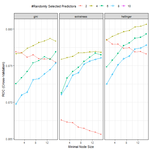
从这个图来看和上面的结果是一样的,mtry = 4, splitrule = hellinger and min.node.size = 15的时候,ROC是最高的,大概0.88多一点。
这个数据是不是很好了呢,还有进步的空间吗?不好说
下面我们对数据做一些常规的预处理,重新建立模型,再看一看效果。
做数据预处理
预处理
首先处理结果变量类不平衡的问题,我们这里就用downsampling吧,这个方法也在之前的推文中铺垫过了:R语言机器学习caret-06:重采样解决类不平衡
hotels <- downSample(x = hotels_df[,-1],
                     y = hotels_df$children,
                     yname = "Children"
                     )
table(hotels$Children)
##
## children     none
##     6073     6073
Class <- hotels$Class

dim(hotels)
## [1] 12146    10
str(hotels)
## 'data.frame':	12146 obs. of  10 variables:
##  $ hotel                      : Factor w/ 2 levels "City Hotel","Resort Hotel": 1 2 1 1 2 1 2 2 1 1 ...
##  $ arrival_date_month         : Factor w/ 12 levels "April","August",..: 6 6 4 3 8 2 6 4 7 1 ...
##  $ meal                       : Factor w/ 5 levels "BB","FB","HB",..: 1 3 1 1 1 1 1 3 1 1 ...
##  $ adr                        : num  185 186 198 0 77 ...
##  $ adults                     : num  2 2 2 2 2 2 3 2 2 2 ...
##  $ required_car_parking_spaces: Factor w/ 2 levels "none","parking": 2 1 1 1 1 2 1 1 1 1 ...
##  $ total_of_special_requests  : num  0 2 1 2 0 0 1 2 2 0 ...
##  $ stays_in_week_nights       : num  1 6 2 2 5 1 5 0 3 2 ...
##  $ stays_in_weekend_nights    : num  2 4 2 0 2 2 2 1 1 0 ...
##  $ Class                      : Factor w/ 2 levels "children","none": 1 1 1 1 1 1 1 1 1 1 ...
这样处理后,结果变量的两个类基本一样多了,但是这个方法损失了很多信息哈,可以看到处理完只剩下12146行了…如果你的数据本身样本量就不大,就不要用这种方法了。
接下来对数值型变量去掉近零方差变量,并进行中心化和标准化,这几个操作可以一起进行:
zcs <- preProcess(hotels,
                  method = c("zv","center", "scale"))
hotels <- predict(zcs, newdata = hotels)
接下来我们对分类变量进行哑变量设置,这个哑变量的我们在之前也提到过很多次了,除了哑变量还有非常多的编码方式,大家感兴趣的去翻历史推文即可。
Children <- hotels$Children
dummy <- dummyVars(Children ~ ., data = hotels)
hotels <- predict(dummy, newdata = hotels)
hotels <- as.data.frame(hotels)
str(hotels)
## 'data.frame':	12146 obs. of  26 variables:
##  $ hotel.City Hotel                   : num  1 0 1 1 0 1 0 0 1 1 ...
##  $ hotel.Resort Hotel                 : num  0 1 0 0 1 0 1 1 0 0 ...
##  $ arrival_date_month.April           : num  0 0 0 0 0 0 0 0 0 1 ...
##  $ arrival_date_month.August          : num  0 0 0 0 0 1 0 0 0 0 ...
##  $ arrival_date_month.December        : num  0 0 0 1 0 0 0 0 0 0 ...
##  $ arrival_date_month.February        : num  0 0 1 0 0 0 0 1 0 0 ...
##  $ arrival_date_month.January         : num  0 0 0 0 0 0 0 0 0 0 ...
##  $ arrival_date_month.July            : num  1 1 0 0 0 0 1 0 0 0 ...
##  $ arrival_date_month.June            : num  0 0 0 0 0 0 0 0 1 0 ...
##  $ arrival_date_month.March           : num  0 0 0 0 1 0 0 0 0 0 ...
##  $ arrival_date_month.May             : num  0 0 0 0 0 0 0 0 0 0 ...
##  $ arrival_date_month.November        : num  0 0 0 0 0 0 0 0 0 0 ...
##  $ arrival_date_month.October         : num  0 0 0 0 0 0 0 0 0 0 ...
##  $ arrival_date_month.September       : num  0 0 0 0 0 0 0 0 0 0 ...
##  $ meal.BB                            : num  1 0 1 1 1 1 1 0 1 1 ...
##  $ meal.FB                            : num  0 0 0 0 0 0 0 0 0 0 ...
##  $ meal.HB                            : num  0 1 0 0 0 0 0 1 0 0 ...
##  $ meal.SC                            : num  0 0 0 0 0 0 0 0 0 0 ...
##  $ meal.Undefined                     : num  0 0 0 0 0 0 0 0 0 0 ...
##  $ adr                                : num  185 186 198 0 77 ...
##  $ adults                             : num  2 2 2 2 2 2 3 2 2 2 ...
##  $ required_car_parking_spaces.none   : num  0 1 1 1 1 0 1 1 1 1 ...
##  $ required_car_parking_spaces.parking: num  1 0 0 0 0 1 0 0 0 0 ...
##  $ total_of_special_requests          : num  0 2 1 2 0 0 1 2 2 0 ...
##  $ stays_in_week_nights               : num  1 6 2 2 5 1 5 0 3 2 ...
##  $ stays_in_weekend_nights            : num  2 4 2 0 2 2 2 1 1 0 ...
进行了这一步操作后预测变量明显变多了~
做完这一套操作后我们的数据变成了12146行和27列:
hotels$Children <- Children
str(hotels)
## 'data.frame':	12146 obs. of  27 variables:
##  $ hotel.City Hotel                   : num  0.815 -1.227 0.815 0.815 -1.227 ...
##  $ hotel.Resort Hotel                 : num  -0.815 1.227 -0.815 -0.815 1.227 ...
##  $ arrival_date_month.April           : num  -0.3 -0.3 -0.3 -0.3 -0.3 ...
##  $ arrival_date_month.August          : num  -0.445 -0.445 -0.445 -0.445 -0.445 ...
##  $ arrival_date_month.December        : num  -0.254 -0.254 -0.254 3.937 -0.254 ...
##  $ arrival_date_month.February        : num  -0.277 -0.277 3.609 -0.277 -0.277 ...
##  $ arrival_date_month.January         : num  -0.229 -0.229 -0.229 -0.229 -0.229 ...
##  $ arrival_date_month.July            : num  2.428 2.428 -0.412 -0.412 -0.412 ...
##  $ arrival_date_month.June            : num  -0.294 -0.294 -0.294 -0.294 -0.294 ...
##  $ arrival_date_month.March           : num  -0.283 -0.283 -0.283 -0.283 3.535 ...
##  $ arrival_date_month.May             : num  -0.296 -0.296 -0.296 -0.296 -0.296 ...
##  $ arrival_date_month.November        : num  -0.216 -0.216 -0.216 -0.216 -0.216 ...
##  $ arrival_date_month.October         : num  -0.291 -0.291 -0.291 -0.291 -0.291 ...
##  $ arrival_date_month.September       : num  -0.272 -0.272 -0.272 -0.272 -0.272 ...
##  $ meal.BB                            : num  0.524 -1.907 0.524 0.524 0.524 ...
##  $ meal.FB                            : num  -0.0829 -0.0829 -0.0829 -0.0829 -0.0829 ...
##  $ meal.HB                            : num  -0.402 2.489 -0.402 -0.402 -0.402 ...
##  $ meal.SC                            : num  -0.254 -0.254 -0.254 -0.254 -0.254 ...
##  $ meal.Undefined                     : num  -0.096 -0.096 -0.096 -0.096 -0.096 ...
##  $ adr                                : num  1.015 1.024 1.225 -1.959 -0.721 ...
##  $ adults                             : num  0.236 0.236 0.236 0.236 0.236 ...
##  $ required_car_parking_spaces.none   : num  -2.539 0.394 0.394 0.394 0.394 ...
##  $ required_car_parking_spaces.parking: num  2.539 -0.394 -0.394 -0.394 -0.394 ...
##  $ total_of_special_requests          : num  -0.976 1.189 0.106 1.189 -0.976 ...
##  $ stays_in_week_nights               : num  -0.803 1.794 -0.284 -0.284 1.274 ...
##  $ stays_in_weekend_nights            : num  1.017 3.022 1.017 -0.988 1.017 ...
##  $ Children                           : Factor w/ 2 levels "children","none": 1 1 1 1 1 1 1
建立模型
方法还是和之前一样的,就不多说了。
# 设定种子数
set.seed(3456)

# 根据结果变量的类别多少划分
trainIndex <- createDataPartition(hotels$Children, p = 0.7,
                                  list = FALSE)
head(trainIndex)
##      Resample1
## [1,]         1
## [2,]         2
## [3,]         3
## [4,]         5
## [5,]         6
## [6,]         7

hotelsTrain <- hotels[ trainIndex,]
hotelsTest  <- hotels[-trainIndex,]

# 选择重抽样方法,10折交叉验证
trControl <- trainControl(method = "cv", number = 10,
                          classProbs = T,
                          summaryFunction = twoClassSummary
                          )

# 网格搜索,首先设定超参数范围
rfGrid <-  expand.grid(mtry = seq(2,10,2),
                       splitrule = c( "gini", "extratrees", "hellinger"),
                       min.node.size = seq(1,15,2)
                       )

# 设置种子数,进行建模
library(doParallel)
cl <- makePSOCKcluster(16)
registerDoParallel(cl)

set.seed(8)

rffit <- train(x = hotelsTrain[,-15],
               y = hotelsTrain$Children,
               method = "ranger",
               trControl = trControl,
               verbose = FALSE,
               #tuneLength = 10
               tuneGrid = rfGrid
               )

rffit
## Random Forest
##
## 8504 samples
##   26 predictor
##    2 classes: 'children', 'none'
##
## No pre-processing
## Resampling: Cross-Validated (10 fold)
## Summary of sample sizes: 7654, 7654, 7654, 7652, 7654, 7653, ...
## Resampling results across tuning parameters:
##
##   mtry  splitrule   min.node.size  ROC  Sens  Spec
##    2    gini         1             1    1     1
##    2    gini         3             1    1     1
##    2    gini         5             1    1     1
##    2    gini         7             1    1     1
##    2    gini         9             1    1     1
##    2    gini        11             1    1     1
##    2    gini        13             1    1     1
##    2    gini        15             1    1     1
##    2    extratrees   1             1    1     1
##    2    extratrees   3             1    1     1
##    2    extratrees   5             1    1     1
##    2    extratrees   7             1    1     1
##    2    extratrees   9             1    1     1
##    2    extratrees  11             1    1     1
##    2    extratrees  13             1    1     1
##    2    extratrees  15             1    1     1
##    2    hellinger    1             1    1     1
##    2    hellinger    3             1    1     1
##    2    hellinger    5             1    1     1
##    2    hellinger    7             1    1     1
##    2    hellinger    9             1    1     1
##    2    hellinger   11             1    1     1
##    2    hellinger   13             1    1     1
##    2    hellinger   15             1    1     1
##    4    gini         1             1    1     1
##    4    gini         3             1    1     1
##    4    gini         5             1    1     1
##    4    gini         7             1    1     1
##    4    gini         9             1    1     1
##    4    gini        11             1    1     1
##    4    gini        13             1    1     1
##    4    gini        15             1    1     1
##    4    extratrees   1             1    1     1
##    4    extratrees   3             1    1     1
##    4    extratrees   5             1    1     1
##    4    extratrees   7             1    1     1
##    4    extratrees   9             1    1     1
##    4    extratrees  11             1    1     1
##    4    extratrees  13             1    1     1
##    4    extratrees  15             1    1     1
##    4    hellinger    1             1    1     1
##    4    hellinger    3             1    1     1
##    4    hellinger    5             1    1     1
##    4    hellinger    7             1    1     1
##    4    hellinger    9             1    1     1
##    4    hellinger   11             1    1     1
##    4    hellinger   13             1    1     1
##    4    hellinger   15             1    1     1
##    6    gini         1             1    1     1
##    6    gini         3             1    1     1
##    6    gini         5             1    1     1
##    6    gini         7             1    1     1
##    6    gini         9             1    1     1
##    6    gini        11             1    1     1
##    6    gini        13             1    1     1
##    6    gini        15             1    1     1
##    6    extratrees   1             1    1     1
##    6    extratrees   3             1    1     1
##    6    extratrees   5             1    1     1
##    6    extratrees   7             1    1     1
##    6    extratrees   9             1    1     1
##    6    extratrees  11             1    1     1
##    6    extratrees  13             1    1     1
##    6    extratrees  15             1    1     1
##    6    hellinger    1             1    1     1
##    6    hellinger    3             1    1     1
##    6    hellinger    5             1    1     1
##    6    hellinger    7             1    1     1
##    6    hellinger    9             1    1     1
##    6    hellinger   11             1    1     1
##    6    hellinger   13             1    1     1
##    6    hellinger   15             1    1     1
##    8    gini         1             1    1     1
##    8    gini         3             1    1     1
##    8    gini         5             1    1     1
##    8    gini         7             1    1     1
##    8    gini         9             1    1     1
##    8    gini        11             1    1     1
##    8    gini        13             1    1     1
##    8    gini        15             1    1     1
##    8    extratrees   1             1    1     1
##    8    extratrees   3             1    1     1
##    8    extratrees   5             1    1     1
##    8    extratrees   7             1    1     1
##    8    extratrees   9             1    1     1
##    8    extratrees  11             1    1     1
##    8    extratrees  13             1    1     1
##    8    extratrees  15             1    1     1
##    8    hellinger    1             1    1     1
##    8    hellinger    3             1    1     1
##    8    hellinger    5             1    1     1
##    8    hellinger    7             1    1     1
##    8    hellinger    9             1    1     1
##    8    hellinger   11             1    1     1
##    8    hellinger   13             1    1     1
##    8    hellinger   15             1    1     1
##   10    gini         1             1    1     1
##   10    gini         3             1    1     1
##   10    gini         5             1    1     1
##   10    gini         7             1    1     1
##   10    gini         9             1    1     1
##   10    gini        11             1    1     1
##   10    gini        13             1    1     1
##   10    gini        15             1    1     1
##   10    extratrees   1             1    1     1
##   10    extratrees   3             1    1     1
##   10    extratrees   5             1    1     1
##   10    extratrees   7             1    1     1
##   10    extratrees   9             1    1     1
##   10    extratrees  11             1    1     1
##   10    extratrees  13             1    1     1
##   10    extratrees  15             1    1     1
##   10    hellinger    1             1    1     1
##   10    hellinger    3             1    1     1
##   10    hellinger    5             1    1     1
##   10    hellinger    7             1    1     1
##   10    hellinger    9             1    1     1
##   10    hellinger   11             1    1     1
##   10    hellinger   13             1    1     1
##   10    hellinger   15             1    1     1
##
## ROC was used to select the optimal model using the largest value.
## The final values used for the model were mtry = 2, splitrule = gini
##  and min.node.size = 1.
结果很明显比不做预处理好多了,ROC直接到1了!而且由于我们用了downsampling,运行速度明显加快。
下面还是画个图更直观的看一下:
ggplot(rffit)+theme_bw()+theme(legend.position = "top")

效果还是很显著的,这样我们就选择一个最简单的模型就可以了。看看caret包为我们自动选择的最终模型:
rffit$finalModel
## Ranger result
##
## Call:
##  ranger::ranger(dependent.variable.name = ".outcome", data = x,      mtry = min(param$mtry, ncol(x)), min.node.size = param$min.node.size,      splitrule = as.character(param$splitrule), write.forest = TRUE,      probability = classProbs, ...)
##
## Type:                             Probability estimation
## Number of trees:                  500
## Sample size:                      8504
## Number of independent variables:  26
## Mtry:                             2
## Target node size:                 1
## Variable importance mode:         none
## Splitrule:                        gini
## OOB prediction error (Brier s.):  0.04232395
查看自动为我们选择的超参数:
rffit$bestTune
##   mtry splitrule min.node.size
## 1    2      gini             1
训练集
然后就可以直接用这个模型在测试集做预测了,我这里直接把测试集的真实类别,预测类别,预测概率放在一个数据框中了,方便进行各种计算和操作。
library(dplyr)
##
## Attaching package: 'dplyr'
## The following objects are masked from 'package:stats':
##
##     filter, lag
## The following objects are masked from 'package:base':
##
##     intersect, setdiff, setequal, union
test_pred <- select(hotelsTest, Children) %>%
  bind_cols(predict(rffit, newdata = hotelsTest,type = "prob")) %>%
  bind_cols(pred = predict(rffit, newdata = hotelsTest))

head(test_pred)
##   Children  children      none     pred
## 4  children 0.7915756 0.2084244 children
## 12 children 0.8770473 0.1229527 children
## 14 children 0.8565740 0.1434260 children
## 19 children 0.7310673 0.2689327 children
## 23 children 0.8696240 0.1303760 children
## 25 children 0.8097900 0.1902100 children
混淆矩阵:
confusionMatrix(data = test_pred$Children, test_pred$pred)
## Confusion Matrix and Statistics
##
##           Reference
## Prediction children none
##   children     1821    0
##   none            0 1821
##
##                Accuracy : 1
##                  95% CI : (0.999, 1)
##     No Information Rate : 0.5
##     P-Value [Acc > NIR] : < 2.2e-16
##
##                   Kappa : 1
##
##  Mcnemar's Test P-Value : NA
##
##             Sensitivity : 1.0
##             Specificity : 1.0
##          Pos Pred Value : 1.0
##          Neg Pred Value : 1.0
##              Prevalence : 0.5
##          Detection Rate : 0.5
##    Detection Prevalence : 0.5
##       Balanced Accuracy : 1.0
##
##        'Positive' Class : children
##
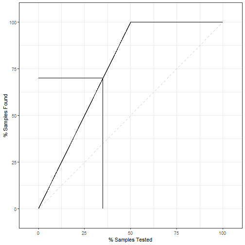
提升曲线:
lift_obj <- lift(Children ~ children, data = test_pred)
ggplot(lift_obj,values = 70)+theme_bw()
校准曲线:
cal_obj <- calibration(Children ~ children, data = test_pred,cuts = 10)
ggplot(cal_obj)+theme_bw()
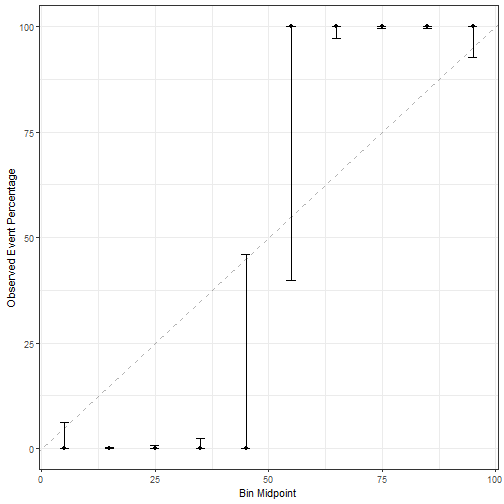
可以看出我们的模型区分度很好,但是校准度一塌糊涂。
多个模型的比较我们之前也演示过了,大家可以参考之前的推文。