Overview
ggplot2 基于the grammar of graphics思想,通过数据集、几何对象和坐标系统建立图形。
所有的ggplot2绘图都以ggplot()开始, 默认由aes()将数据集映射至几何对象。在行尾+添加图层:几何,比例尺,坐标和面等。要将绘图保存,请使用ggsave()
完整的ggplot2图形包括:
-
ggplot(data,aes(...)): Create a new ggplot (required)
-
geom_<FUNC>(aes(...),data,stat,position): Geometric object (required)
or stat_<FUNC>(aes(...),data,geom,position): Statistical transformation (required)
-
coord_<FUNC>(...): Coordinate systems
-
facet_<FUNC>(...): Facetting
-
scale_<FUNC>(...): Scales
-
theme_<FUNC>(...): Themes
data, aes参数可以在ggplot, geom_<FUNC>, stat_<FUNC>任一函数中加载
aes() 控制数据中的变量映射到几何图形。aes()映射可以在ggplot()和geom图层中设置。常用参数:alpha, color, group, linetype, size
ggsave(filename, plot = last_plot(),path=NULL,width, height, units= c("in", "cm", "mm"))保存ggplot2图形,默认保存最后一个图
qplot(),quickplot(): Quick plot
Geoms
用geom函数表现图形,geom中的aes参数映射数据,每一个geom函数添加一个图层。
| geom常用几何参数 |
常量赋值 |
| color/fill |
color/fill=NA 消除线条或填充 |
| alpha |
0 <= alpha <= 1 |
| linetype |
线条形式(1:6) |
| size |
点的尺寸和线的宽度 |
| shape |
点的形状(0:25) |
基本图形
| 函数 |
参数 |
说明 |
| geom_blank() |
|
空白 |
geom_curve(aes(yend,xend,curvature))
geom_segment(aes(yend,xend)) |
x, xend, y, yend, alpha, angle, color, curvature(曲率), linetype, size, arrow |
曲线
线段 |
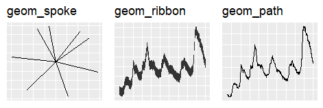
| geom_path(lineend, linejoin, linemitre) |
x, y, alpha, color, group, linetype, size(x为分类变量时必须设置group=1) |
路径 |
| geom_polygon(aes(group)) |
x, y, alpha, color, fill, group, linetype, size |
多边形 |
| geom_rect(aes(xmin, ymin, xmax, ymax)) |
xmax, xmin, ymax, ymin, alpha, color, fill, linetype, size |
矩形 |
| geom_ribbon(aes(ymin, ymax)) |
x, ymax, ymin, alpha, color, fill, group, linetype, size |
丝带图 |
| geom_abline(aes(intercept, slope)) |
x, y, alpha, color, linetype, size |
斜线 |
| geom_hline(aes(yintercept)) |
x, y, alpha, color, linetype, size |
水平线 |
| geom_vline(aes(xintercept)) |
x, y, alpha, color, linetype, size |
垂直线 |
| geom_segment(aes(yend, xend)) |
x, y, alpha, color, linetype, size |
线段 |
| geom_spoke(aes(angle, radius)) |
x, y, alpha, color, linetype, size |
辐条 |
them_blank <- theme(axis.text=element_blank(),
                 axis.title = element_blank()
                 axis.ticks=element_blank())

p1=ggplot()+
  geom_spoke(aes(x=0,y=0,angle = 1:8, radius = 5))+
  them_blank+
  ggtitle('geom_spoke')
a <- ggplot(economics, aes(date, unemploy))
a + geom_ribbon(aes(ymin=unemploy - 900, ymax=unemploy + 900))+
  them_blank+
  ggtitle('geom_ribbon')
a + geom_path(lineend="butt", linejoin="round", linemitre=1)+
  them_blank+
  ggtitle('geom_path')
单变量
stat参数 : bin/count/identity
- 若x为连续变量:stat= ”bin”
- 若x离散变量:stat = “count”或stat = “identity”
| continuous |
参数 |
说明 |
| geom_area() |
x, y, alpha, color, fill, linetype, size,stat={identity,bin} |
面积图 |
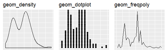
| geom_density(kernel = “gaussian”) |
x, y, alpha, color, fill, group, linetype, size, weight, adjust=1/2(调整带宽倍率), stat={density,count,scaled (密度估计值)} |
核密度图 |
| geom_dotplot() |
x, y, alpha, color, fill |
点状分布图 |
| geom_freqpoly() |
x, y, alpha, color, group, linetype, size |
频率多边形(类似直方图) |
| geom_histogram(binwidth) |
x, y, alpha, color, fill, linetype, size, weight |
直方图 |
| geom_qq(aes(sample)) |
x, y, alpha, color, fill, linetype, size, weight |
qq图(检测正态分布) |
| discrete |
|
|
| geom_bar() |
x, alpha, color, fill, linetype, size, weight, stat={count,prop (分组比例)} |
柱状图 |
c <- ggplot(mpg, aes(hwy)); c2 <- ggplot(mpg)
c + geom_density()+
  them_blank+
  ggtitle('geom_density')
c + geom_dotplot() +
  them_blank+
  ggtitle('geom_dotplot')
c + geom_freqpoly()+
  them_blank+
  ggtitle('geom_freqpoly')
双变量
continuous x
continuous y |
参数 |
说明 |
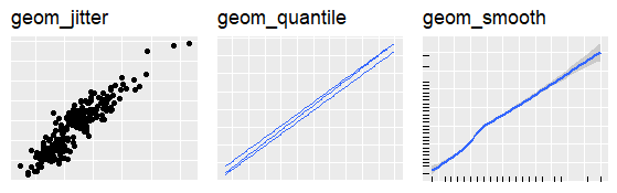
| geom_jitter(height , width) |
x, y, alpha, color, fill, shape, size |
抖点图(避免重合),stat = “identity” |
| geom_point() |
x, y, alpha, color, fill, shape, size, stroke |
散点图stat = “identity” |
| geom_quantile() |
x, y, alpha, color, group, linetype, size, weight |
四分位图 |
| geom_rug(sides) |
x, y, alpha, color, linetype, size,sides(地毯位置) |
地毯图 |
| geom_smooth() |
x, y, alpha, color, fill, group, linetype, size, weight |
拟合曲线,自动计算变量:y/ymin/ymax/se(标准误) |
geom_smooth(method = "auto", formula = y ~ x)
参数:
method: eg. “lm”, “glm”, “gam”, “loess”, “rlm”
formula :eg. y ~ x, y ~ poly(x, 2), y ~ log(x)
se : 是否绘制置信区间(默认为TRUE)
level : 用的置信区间水平(默认为95%)
if(!require(quantreg)) install.packages("quantreg")#四分位图必须的包
e <- ggplot(mpg, aes(cty, hwy))
e + geom_jitter(height = 2, width = 2)  +
  them_blank+
  ggtitle('geom_jitter')
e + geom_quantile() +
  them_blank+
  ggtitle('geom_quantile')
e + geom_smooth()+
  geom_rug(sides = "bl")+
  them_blank+
  ggtitle('geom_smooth')
| 两连续变量分布图 |
参数 |
说明 |
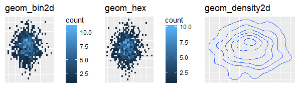
| geom_density2d() |
x, y, alpha, colour, group, linetype, size, fill=…level…(自动计算变量) |
分布密度 |
| geom_bin2d(binwidth) |
x, y, alpha, color, fill, linetype, size, weight |
矩形箱,stat = “bin2d” |
| geom_hex() |
x, y, alpha, colour, fill, size |
六角仓,stat = “binhex” |
if(!require(hexbin)) install.packages("hexbin")#六角仓必须的包
df <- data.frame(x=rnorm(1000,0,100),y=rnorm(1000,10,50))

h <- ggplot(df, aes(x, y))
h + geom_bin2d() +
  them_blank+
  ggtitle('geom_bin2d')
h + geom_hex()+
  them_blank+
  ggtitle('geom_hex')
h + geom_density2d() +
  them_blank+
  ggtitle('geom_density2d')
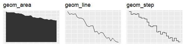
| 两连续变量函数图 |
参数 |
说明 |
| geom_area() |
x, y, alpha, color, fill, linetype, size |
面积图 |
| geom_line() |
x, y, alpha, color, group, linetype, size |
折线图 |
| geom_step(direction = “hv”) |
x, y, alpha, color, group, linetype, size |
阶梯图 |
recent <- economics[economics$date > as.Date("2013-01-01"), ]
p <- ggplot(recent, aes(date, unemploy))

p + geom_area() +
  them_blank+
  ggtitle('geom_area')
p + geom_line()+
  them_blank+
  ggtitle('geom_line')
p + geom_step(direction = "hv") +
  them_blank+
  ggtitle('geom_step')
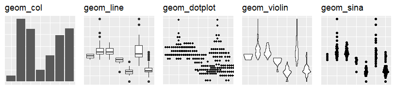
discrete x
continuous y |
参数 |
说明 |
| geom_col() |
x, y, alpha, color, fill, group, linetype, size |
柱状图 |
| geom_boxplot() |
x, y, lower, middle, upper, ymax, ymin, alpha, color, fill, group, linetype, shape, size, weight, notch(是否缺口), width,outlier |
箱线图 |
| geom_dotplot(binaxis = “y”, stackdir = “center”) |
x, y, alpha, color, fill, group |
点状分布图(不重合) |
| geom_violin(scale = “area”) |
x, y, alpha, color, fill, group, linetype, size, weight |
小提琴图 |
| ggforce::geom_sina() |
|
点状小提琴图 |
p <-  ggplot(mpg, aes(class, hwy))

p +geom_col() +
  them_blank+
  ggtitle('geom_col')
p +geom_boxplot()+
  them_blank+
  ggtitle('geom_line')
p +geom_dotplot(binaxis = "y", stackdir = "center") +
  them_blank+
  ggtitle('geom_dotplot')
p +geom_violin(scale = "area")+
  them_blank+
  ggtitle('geom_violin')
p +ggforce::geom_sina()+
  them_blank+
  ggtitle('geom_sina')
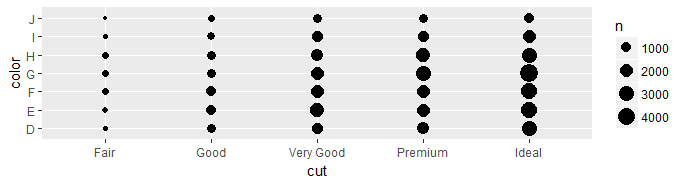
discrete x
discrete y |
参数 |
说明 |
| geom_count() |
x, y, alpha, color, fill, shape, size, stroke |
计数图 |
ggplot(diamonds, aes(cut, color))+
  geom_count()
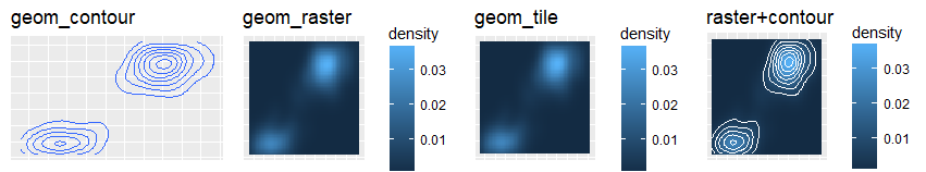
三变量
| 函数 |
参数 |
说明 |
| geom_contour(aes(z)) |
x, y, z, alpha, colour, group, linetype, size, weight,bins(等高线数量),binwidth(等高线宽度) |
等高线图, …level…(轮廓高度,自动计算变量) |
| geom_raster(aes(fill)) |
x,y,alpha,fill |
光栅(热力图) |
| geom_tile(aes(fill)) |
x, y, alpha, color, fill, linetype, size, width |
瓦片(热力图) |
p <-  ggplot(faithfuld, aes(waiting, eruptions))

p +geom_contour(aes(z = density)) +
  them_blank+
  ggtitle('geom_contour')
p +geom_raster(aes(fill = density), hjust=0.5, vjust=0.5, interpolate=FALSE) +
  them_blank+
  ggtitle('geom_raster')
p + geom_tile(aes(fill = density)) +
  them_blank+
  ggtitle('geom_tile')
p + geom_raster(aes(fill = density)) +
  geom_contour(aes(z = density),colour = "white")+
  them_blank+
  ggtitle('raster+contour') #图层顺序很重要
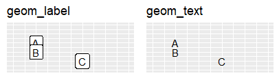
文本
| 函数 |
参数 |
说明 |
| geom_text(aes(label), nudge_x, nudge_y, check_overlap = TRUE) |
x, y, label, alpha, angle, color, family, fontface, hjust, lineheight, size, vjust |
|
| geom_label(aes(label), nudge_x, nudge_y, check_overlap = TRUE) |
x, y, label, alpha, angle, color, family, fontface, hjust, lineheight, size, vjust |
有背景框 |
参数:
nudge_x, nudge_y: 微调
check_overlap:是否过重叠
vjust,hjust: 对齐方式(0:1)
angle: 角度
lineheight:行间距
family: 字体
size: 字体大小
fontface: 字体格式(1:4, plain标准,bold加粗,italic斜体,bold.italic)
ggrepel包 : 文字不重叠
ggrepel:: geom_label_repel()
ggrepel:: geom_text_repel()
df=data.frame(x=c(1,1,3),y=c(3,2,1),t=c('A','B','C'))

e=ggplot(df,aes(x,y))
e + geom_label(aes(label = t)) +
  them_blank+lims(x=c(0,5),y=c(0,5))+
  ggtitle('geom_label')
e + geom_text(aes(label = t)) +
  them_blank+lims(x=c(0,5),y=c(0,5))+
  ggtitle('geom_text')
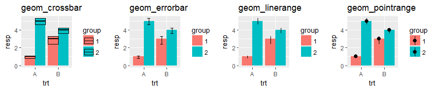
误差可视化
| 函数 |
参数 |
说明 |
| geom_crossbar(fatten) |
x, y, ymax, ymin, alpha, color, fill, group, linetype, size |
|
| geom_errorbar() |
x, ymax, ymin, alpha, color, group, linetype, size, width (also geom_errorbarh()) |
|
| geom_linerange() |
x, ymin, ymax, alpha, color, group, linetype, size |
|
| geom_pointrange() |
x, y, ymin, ymax, alpha, color, fill, group, linetype, shape, size |
|
aes(ymin,ymax) : ymin,ymax需要在aes参数内赋值
df <- data.frame(
  trt = factor(c('A', 'A', 'B', 'B')),
  resp = c(1, 5, 3, 4),
  group = factor(c(1, 2, 1, 2)),
  upper = c(1.1, 5.3, 3.3, 4.2),
  lower = c(0.8, 4.6, 2.4, 3.6)
)

dodge <- position_dodge(width=0.9) #位置微调
p <- ggplot(df, aes(trt, resp, fill = group,ymin = lower, ymax = upper))+
  geom_col(position = dodge)

p + geom_crossbar(fatten = 2,position = dodge) +
  ggtitle('geom_crossbar')
p + geom_errorbar(position = dodge, width = 0.25) +
  ggtitle('geom_errorbar')
p +geom_linerange(position = dodge) +
  ggtitle('geom_linerange')
p +geom_pointrange(position = dodge) +
  ggtitle('geom_pointrange')
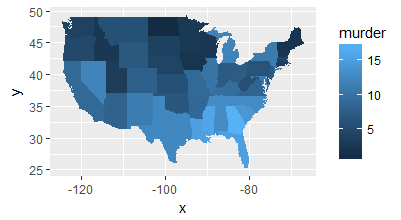
地图
| 函数 |
参数 |
说明 |
| geom_map(aes(map_id), map) |
map_id, alpha, color, fill, linetype, size |
地图 |
参数:
map_id:id/region
map: data.frame(x/long, y/lat, id/region) 或sp空间数据
Tips:
sf::st_read 读取sp或json文件
sf::st_transform 转换sf文件
地图素材:
矢量地图素材链接
shp数据地图:GitHub ,GADM
Json数据地图:阿里云, 百度Echarts
if(!require(maps)) install.packages("maps") # 载入地图包(版本过老)
data <- data.frame(murder = USArrests$Murder,state = tolower(rownames(USArrests)))

map <- maps::map_data("state")
ggplot(data, aes(fill = murder))+
  geom_map(aes(map_id = state), map = map) +
  expand_limits(x = map$long, y = map$lat)
Stats
ggplot2还提供一种替代方案,建立一个图层用stat计算新变量 (e.g., count, prop)作图。
- 改变geom函数的stat默认值,如
geom_bar(stat="count")
- 调用
stat_<FUNC>,如 stat_count(geom="bar")
- 用
..name..的语法格式,将stat计算变量映射到几何对象,如stat_density2d(aes(fill = ..level..), geom = "polygon")
| 函数 |
参数 |
计算变量 |
说明 |
| stat_bin(binwidth, origin) |
x, y |
…count…, …ncount…, …density…, …ndensity… |
|
| stat_count(width = 1) |
x, y |
…count…, …prop… |
|
| stat_density(adjust = 1, kernel = “gaussian") |
x, y |
…count…, …density…, …scaled… |
|
| ------ |
------ |
------ |
------ |
| stat_bin_2d(bins, drop = TRUE) |
x, y, fill |
…count…, …density… |
|
| stat_bin_hex(bins) |
x, y, fill |
…count…, …density… |
|
| stat_density_2d(contour = TRUE, n = 100) |
x, y, color, size |
…level… |
|
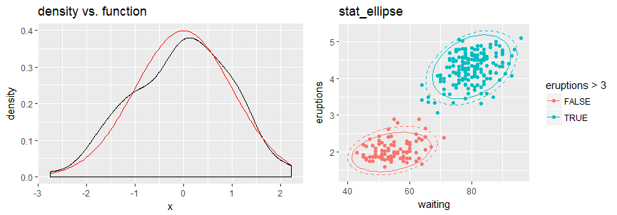
| stat_ellipse(level, segments, type = “t”) |
|
|
计算正常置信度椭圆 |
| ------ |
------ |
------ |
------ |
| stat_contour(aes(z)) |
x, y, z, order |
…level… |
|
| stat_summary_hex(aes(z), bins, fun = max) |
x, y, z, fill |
…value… |
六边形 |
| stat_summary_2d(aes(z), bins, fun = mean) |
x, y, z, fill |
…value… |
矩形 |
| stat_boxplot(coef) |
x, y |
…lower…, …middle…, …upper…, …width… , …ymin…, …ymax… |
|
| stat_ydensity(kernel = “gaussian”, scale = “area") |
x, y |
…density…, …scaled…, …count…, …n…, …violinwidth…, …width… |
|
| ------ |
------ |
------ |
------ |
| stat_ecdf(n) |
x, y |
…x…, …y… |
计算经验累积分布 |
| stat_quantile(quantiles = c(0.1, 0.9), formula = y ~ log(x), method = “rq”) |
x, y |
…quantile… |
|
| stat_smooth(method = “lm”, formula = y ~ x, se=T, level=0.95) |
x, y |
…se…, …x…, …y…, …ymin…, …ymax… |
|
| ------ |
------ |
------ |
------ |
| stat_function(aes(x = -3:3), n = 99, fun = dnorm, args = list(sd=0.5)) |
x |
…x…, …y… |
计算每个x值的函数 |
| stat_identity(na.rm = TRUE) |
|
|
保持原样 |
| stat_qq(aes(sample=1:100), dist = qt, dparam=list(df=5)) |
sample, x, y |
…sample…, …theoretical… |
|
| stat_sum() |
x, y, size |
…n…, …prop… |
|
| stat_summary(fun.data = “mean_cl_boot”) |
|
|
将y值汇总在唯一x中 |
| stat_summary_bin(fun.y = “mean”, geom = “bar”) |
|
|
将y值汇总在分箱x中 |
| stat_unique() |
|
|
删除重复项 |
set.seed(1492)
df <- data.frame(
  x = rnorm(100)
)
ggplot(df, aes(x)) + geom_density()+
  stat_function(fun = dnorm, colour = "red")+
  ggtitle('density vs. function')

ggplot(faithful, aes(waiting, eruptions, color = eruptions > 3)) +
  geom_point() +
  stat_ellipse(type = "norm", linetype = 2) +
  stat_ellipse(type = "t")+
  ggtitle('stat_ellipse')
Scales
Scales传递数据给几何对象,改变图形的默认标尺。
p <- ggplot(mpg, aes(fl)) +
  geom_bar(aes(fill = fl))

p + scale_fill_manual(
# scale: scale, fill: 几何对象, manual: 预处理的scale类型
  values = c("skyblue", "royalblue", "blue","navy"), #scale参数
  limits = c("d", "e", "p", "r"), #限制范围
  breaks =c("d", "e", "p", "r"), #breaks to use in legend/axis
  labels = c("D", "E", "P", "R"), #labels to use in legend/axis
  name = "fuel") #legend/axis 标题

常用标尺格式
type: color,size,fill,shape,linetype,alpha,etc
scale_<type>_continuous() #连续变量映射
scale_<type>_discrete() #离散变量映射
scale_<type>_identity() #原始数据直接映射
scale_<type>_manual(value=c(…)) #自定义值范围
坐标轴标尺
| X & Y location scales |
说明 |
| lims(x,y)/xlim()/ylim() |
|
| scale_x_continuous(breaks, labels,limits) |
刻度,标签,值的范围 |
| scale_x_discrete(breaks, labels,limits) |
|
| scale_x_date(date_breaks , date_labels) |
日期间隔(“2 weeks”),日期显示格式(%m/%d) |
| scale_x_datetime() |
时间日期,参数同date |
| scale_x_log10() |
log10 标尺 |
| scale_x_reverse() |
x轴方向颠倒 |
| scale_x_sqrt() |
|
Color and fill scales
| Continuous |
说明 |
| scale_fill_distiller(palette = “Blues”) |
|
| scale_fill_gradient(low,high) |
渐变色调控 |
| scale_fill_gradient2(low,mid,high,midpoint) |
2极渐变色 |
| scale_fill_gradientn(values) |
n极渐变色 |
| Discrete |
|
| scale_fill_hue() |
离散色阶 |
| scale_fill_brewer(palette = “Blues”) |
调色板 |
| scale_fill_grey(start, end) |
灰色调 |
调色板离散色阶palette选择:
RColorBrewer::display.brewer.all()
连续色阶选择:
Also: rainbow(), heat.colors(), terrain.colors(), cm.colors()
RColorBrewer::brewer.pal()
#离散色阶
p <- ggplot(mpg, aes(fl)) +
geom_bar(aes(fill = fl))
p +scale_fill_brewer(palette = "Blues")+
ggtitle('scale_fill_brewer')
p + scale_fill_grey(start = 0.2, end = 0.8,na.value = "red") +
ggtitle('scale_fill_grey')
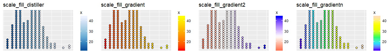
#连续色阶
p <- ggplot(mpg, aes(hwy))+
geom_dotplot(aes(fill = ..x..))
p + scale_fill_distiller(palette = "Blues") +
ggtitle('scale_fill_distiller')
p + scale_fill_gradient(low="red", high="yellow") +
ggtitle('scale_fill_gradient')
p + scale_fill_gradient2(low="red", high="blue", mid = "white", midpoint = 25) +
ggtitle('scale_fill_gradient2')
p +scale_fill_gradientn(colours=topo.colors(6)) +
ggtitle('scale_fill_gradientn')

Shape and size scales
| shape |
说明 |
| scale_shape() |
形状 |
| scale_shape_manual(values) |
|
| size |
|
| scale_size() |
大小 |
| scale_radius(range) |
半径 |
shape:

df <- data.frame(x=1:10,y=sample(1:10,10),
                 s1=rnorm(10),
                 s2=sample(1:4,10,replace = TRUE))
p <- ggplot(df, aes(x, y))+
  geom_point(aes(shape = factor(s2), size = s1, color=factor(s2)))
p + scale_shape_manual(values = c(3:7))
p + scale_radius(range = c(1,6))
Coordinate Systems
| Coordinate Systems |
参数 |
说明 |
| coord_cartesian() |
xlim,ylim |
笛卡尔坐标(默认) |
| coord_fixed() |
radio,xlim,ylim |
具有固定纵横比的直角坐标 |
| coord_flip |
xlim,ylim |
x和y翻转(笛卡尔坐标) |
| coord_polar |
theta, start, direction |
极坐标 |
| coord_trans() |
xtrans, ytrans,xlim,ylim |
变换笛卡尔坐标系,xtrans, ytrans接收函数名 |
coord_quickmap()
coord_map(projection = “ortho”,orientation ) |
projection, orienztation, xlim, ylim |
地图投影 projections:{mercator (default), azequalarea, lagrange, etc.} |
ggplot(mpg, aes(fl)) + them_blank+
  geom_bar()+
  coord_polar(theta = "x", direction=1)

world <- map_data("world")
worldmap <- ggplot(world, aes(x = long, y = lat, group = group)) +
  geom_path() +
  scale_y_continuous(breaks = (-2:2) * 30) +
  scale_x_continuous(breaks = (-4:4) * 45)
worldmap + coord_map("ortho", orientation = c(41, -74, 0))


Position Adjustments
Position adjustments 对geoms进行位置调整。
geom参数赋值字符串
字符串: identity,jitterdodge (同时闪避和抖动),nudge(微距点固定距离)
| geom |
position |
| geom_bar/aera/density |
dodge(并排), stack/fill(堆叠) |
| geom_point |
jitter(减少点重叠) |
| geom_label |
nudge(轻推来自点的标签) |
geom参数赋值position函数
| position函数 |
说明 |
| position_dodge(width) |
抖动宽度(geom默认width=0.9,调用此函数时,width应设为0.9) |
| position_identity() |
不调整 |
| position_jitter(width , height ) |
|
| position_jitterdodge() |
|
| position_nudge(x = 0, y = 0) |
平移距离 |
| position_stack(vjust = 1) |
对齐方式 |
| position_fill(vjust = 1) |
|
p <- ggplot(mpg, aes(fl, fill = drv))

p +  geom_bar(position = "dodge")+
  ggtitle('position = "dodge"')
p +  geom_bar(position = "fill")+
  ggtitle('position = "fill"')
p +   geom_bar(position = "stack")+
  ggtitle('position = "stack"')

Themes
theme(…)
设置主题包括title,axis,legend, panel, background,etc
| 主题函数 |
说明 |
| theme_bw(base_size,base_family) |
黑白主题 |
| theme_grey() |
灰色主题(默认) |
| theme_dark() |
黑色主题 |
| theme_void() |
空主题 |
| theme_minimal() |
最小主题 |
| ggtech::theme_tech() |
技术主题 |
控制theme元素函数(作为主题组件的参数出现):
| 元素函数 |
说明 |
| element_blank |
清空 |
| element_rect(fill,color,size,linetype) |
边框和背景 |
| element_text(family,face, color, size,hjust, vjust,angle,lineheight, margin, debug) |
文字,参数:lineheight(行高), margin(边缘), debug(是否矩形背景) |
| element_line(color,size,linetype,lineend,arrow) |
Line end style (round, butt, square),添加箭头: grid::arrow(angle,length,ends=“last”/“first”/“both”) |
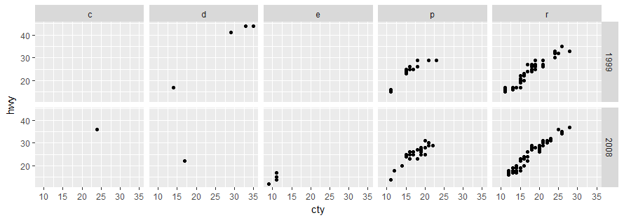
Faceting
刻面通过类别变量将图形分块显示。
| 刻面函数 |
说明 |
| facet_grid(var.row~var.col,scales,labeller) |
网格图,单变量时var.row或var.col用点填充 |
| facet_wrap(~var+var,nrow,ncol,scales,labeller) |
将1d的面板卷成2d网格(nrow*ncol) |
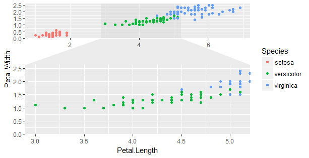
| ggforce::facet_zoom(x, y, xy, split = FALSE, zoom.size = 2) |
子集zoom,x,y,xy 赋值(逻辑值):选取x轴,y轴,xy交叉子集 |
t <- ggplot(mpg, aes(cty, hwy)) + geom_point()
t + facet_grid(year ~ fl)

# ggforce::facet_zoom
ggplot(iris, aes(Petal.Length, Petal.Width, colour = Species)) +
    geom_point() +
    ggforce::facet_zoom(x = Species == "versicolor")
**scales参数:**坐标刻度自由
“fixed”(default,坐标尺度统一), “free”(坐标尺度自由),“free_x”,“free_y”
labeller参数: 调整刻面标签

Annotations and Labels
| Labels |
说明 |
| ggtitle(label, subtitle = NULL) |
图标题 |
| labs(x,y,title,subtitle,caption) |
x/y轴标题 |
| xlab(label)/ylab(label) |
x/y轴标题 |
| Annotations |
说明 |
| annotate(geom,…) |
geom注释,其余参数为geom参数 |
| annotate(“text”,x,y,label, parse=FALSE) |
文本注释 |
| annotate(“pointrange”, x , y, ymin, ymax) |
|
| annotate(“rect”, xmin, xmax, ymin, ymax) |
矩形注释 |
| annotate(“segment”,x, xend, y, yend, arrow) |
线段注释 |
文本注释参数parse:是否数学表达式, 更多公式语法可参考?plotmath
线段注释参数arrow: 添加箭头grid::arrow(angle,length,ends=”last” / ”first”/”both”)
Legends
theme(legend.position = "none"/"bottom"/"top"/"left"/"right") 在主题中设置 Legend
guides(…)设置legends几何组件:colorbar, legend, or none (no legend)
| guide函数 |
作为scale或guides()的参数设置 |
| guide_colorbar(title,label…) |
连续型变量 |
| guide_legend(title,label…) |
离散型变量 |
Vector helpers
| 函数 |
说明 |
| stats::recoder(x_char,x_num,order=FALSE) |
重排序,返回factor/ord.factor |
| cut_interval(x,n,length) |
n组有相同宽度的观测值 |
| cut_number(x,n) |
n组有相同数量的观测值 |
| cut_width(x,width,center,boundary, closed = c(“right”,“left”)) |
|
混合图
gridExtra包可以将多个ggplot2对象组合到一张图中
gridExtra::grid.arrange(plot1,plot2,…,nrow,ncol)
ggplot2 now has an official extension mechanism. This means that others can now easily create their own stats, geoms and positions, and provide them in other packages. This should allow the ggplot2 community to flourish, even as less development work happens in ggplot2 itself. This page showcases these extensions.