本文为自学总结整理知识点使用
参考课程 :
Speech Enhancement :DNN based Spectrum Mapping
传统语音增强方案:谱减法、维纳滤波、MMSE、子空间分解,一般所处理的对象只有一条语音,能学习的特征非常少,这样我们只能通过一些假设(比如:语音或者噪声满足高斯分布;语音于噪声之间相互独立不相关等等)来假定语音的一些特征,并提出一些统计方法,最终设计一些滤波器等方法来进行处理。
随着神经网络技术的不断发展,大量的数据集以及处理能力,不再让我们需要亲自做一些特定假设或者统计特征,而是通过深度神经网络来学习大量语音的特征。
这类方法主要可以分成两大类,一个是 DNN 频谱映射 的方案(关键词 Mapping),一个是 DNN 频谱掩蔽 (关键词:mask )的方法
从大量语音中学习到干净语音的频谱特征
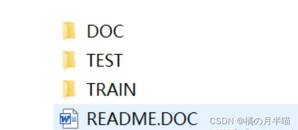
所以要收集大量干净的语音,使用TIMIT数据库,这个数据库组要用于英文的语音识别
打开目录分别表示不同地区;说话人;不同语音的wav文件,采样率16k,以及文本等
因为只做语音增强,所以文本文件可以不要了,只需要,wav文件,
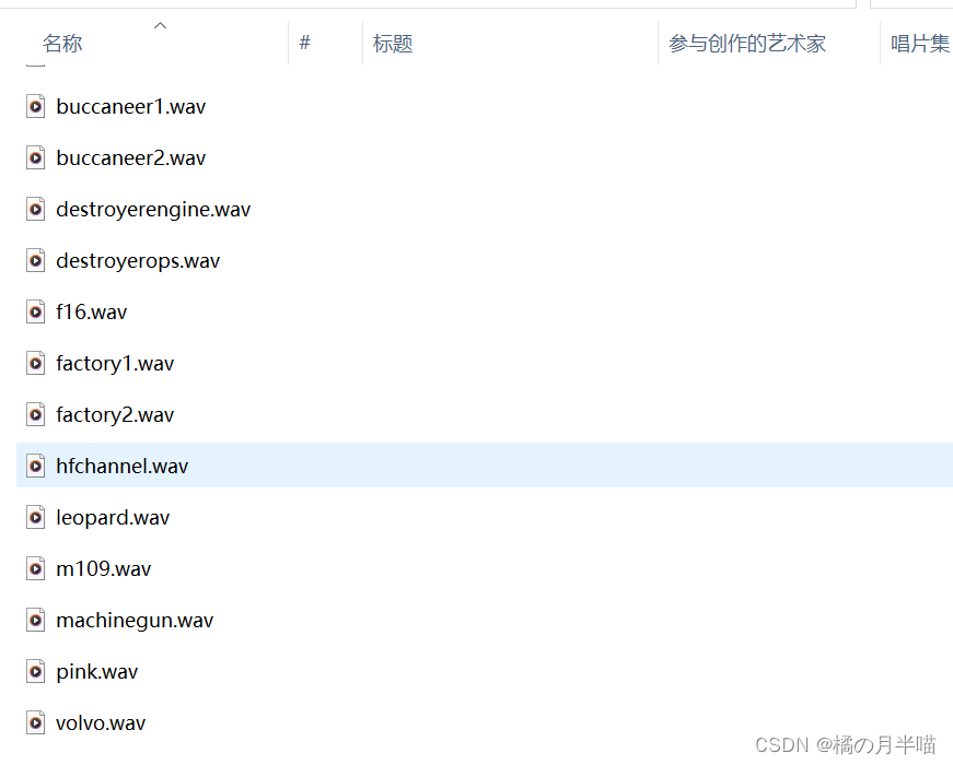
包含15种噪声
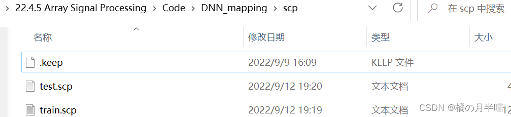
遍历TIMIT,TRAIN文件夹中的所有wav文件,保存 打印文件名到triain.scp文件中。
# get_scp.py
from asyncore import write
import os
from turtle import end_fill
import numpy as np
write_path= "E:\\……\DNN_mapping\\scp"
read_path= "E:\\……\\TIMITdataset"
os. chdir( read_path)
base_path= "TRAIN"
with open ( write_path+ "\\train.scp" , "wt" , encoding= 'utf-8' ) as f:
#base_path="TEST"
#with open(write_path+"\\test.scp","wt",encoding='utf-8') as f:
for root, dirs, files in os. walk( base_path) : #通过 walk函数遍历文件夹中所有文件
# root 表示当前正在访问的文件夹路径
# dirs 表示该文件夹下的子目录名list
# files 表示该文件夹下的文件list
for file in files:
file_name= os. path. join( root, file )
if file_name. endswith( ".WAV" ) :
print ( file_name)
f. write( "%s\n" % file_name)
print ( "done" )
执行分别执行完上述代码之后,会生成两个文件“train.scp”和“test.scp”
主要利用signal_by_db函数产生
根据信噪比定义:
S
N
R
(
d
B
)
=
10
l
o
g
10
(
P
s
i
g
n
a
l
P
n
o
i
s
s
e
)
=
20
l
o
g
20
(
A
s
i
g
n
a
l
A
n
o
i
s
e
)
SNR(dB)=10log_{10}(\frac{P_{signal}}{P_{noisse}})=20log_{20}(\frac{A_{signal}}{A_{noise}})
SNR ( d B ) = 10 l o g 10 ( P n o i sse P s i g na l ) = 20 l o g 20 ( A n o i se A s i g na l )
N
a
d
d
=
n
o
r
m
S
1
0
S
N
R
20
N
n
o
r
m
N
N_{add}=\frac{normS}{10^{\frac{SNR}{20}}}\frac{N}{normN}
N a dd = 1 0 20 SNR n or m S n or m N N
n
o
r
m
X
=
∣
∣
X
∣
∣
2
=
∑
1
N
X
i
2
相当于求幅度值
norm \bold X=|| \bold X||_2=\sqrt {\sum_1^N X_i^2}\quad 相当于求幅度值
n or m X = ∣∣ X ∣ ∣ 2 = 1 ∑ N X i 2
相当于求幅度值
## generate_training.py
import os
import numpy as np
import random
import scipy. io. wavfile as wav
import librosa
import soundfile as sf
from numpy. linalg import norm
def signal_by_db ( speech, noise, snr) :
# 为干净语音加噪声
speech = speech. astype( np. int16)
noise = noise. astype( np. int16)
len_speech = speech. shape[ 0 ] #读取数据常数
len_noise = noise. shape[ 0 ] # 噪声数据的长度要比语音长
start = random. randint( 0 , len_noise- len_speech) # 所以,一般可以随机截取噪声数据 于纯净语音数据相加
end = start+ len_speech
add_noise = noise[ start: end]
# 此处为加噪部分,按照SNR(db)=10log(Ps/Pn)=20log(log(As/An))得来
add_noise = add_noise/ norm( add_noise) * norm( speech) / ( 10.0 ** ( 0.05 * snr) )
mix = speech + add_noise
return mix
if __name__ == "__main__" :
# 噪声数据目录
noise_path = 'E:\\……\\NoiseX-92'
clean_path = "E:\\……\\TIMITdataset" # 干净语音存放目录
scp_path= "E:\\……\\DNN_mapping\\scp"
work_path= "E:\\……\\DNN_mapping"
# 噪声类型 在处理过程中最难处理的就是白噪声和babble噪声,
noises = [ 'babble' , 'buccaneer1' , 'white' ]
os. chdir( work_path)
clean_wavs = np. loadtxt( scp_path+ '\\train.scp' , dtype= 'str' ) . tolist( ) # 读取干净语音的名称,转换成列表
snrs = [ - 5 , 0 , 5 , 10 , 15 , 20 ]
with open ( 'scp/train_DNN_enh.scp' , 'wt' ) as f:
for noise in noises:
print ( noise) #读取噪声数据
noise_file = os. path. join( noise_path, noise+ '.wav' )
noise_data, fs = sf. read( noise_file, dtype = 'int16' )
# 注意,这里采用sf.read 读取成十六进制整数; 若采用librosa.load()读取会自动转换成[-1,+1]之间的浮点数
for clean_wav in clean_wavs: #读取干净语音数据
clean_file = os. path. join( clean_path, clean_wav)
clean_data, fs = sf. read( clean_file, dtype = 'int16' )
for snr in snrs: # 遍历所有SNR
noisy_file = os. path. join( noise_path, noise, str ( snr) , clean_wav) # 加噪数据存放路径,名称
noisy_path, _ = os. path. split( noisy_file)
os. makedirs ( noisy_path, exist_ok= True )
mix = signal_by_db( clean_data, noise_data, snr) # 加噪声
noisy_data = np. asarray( mix, dtype= np. int16) # 保存成 int16格式
sf. write( noisy_file, noisy_data, fs)
f. write( '%s %s\n' % ( noisy_file, clean_file) ) # 存放噪声对名称
# print('%s %s\n'%(noisy_file,clean_file))
整体网络模型通过pytorch实现
# hparams.py
import torch
class hparams ( ) :
def __init__ ( self) :
self. file_scp = "E:\\……\\DNN_mapping\\scp\\train_DNN_enh.scp"
# 训练用的含噪声数据和干净数据数据对
self. para_stft = { }
self. para_stft[ "N_fft" ] = 512
self. para_stft[ "win_length" ] = 512
self. para_stft[ "hop_length" ] = 128
self. para_stft[ "window" ] = 'hamming'
# 网络模型相关参数
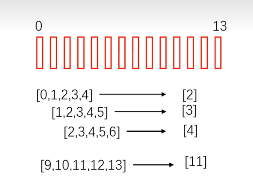
self. n_expand = 3 # 训练时 以多少帧数据作为输入
self. dim_in = int ( ( self. para_stft[ "N_fft" ] / 2 + 1 ) * ( 2 * self. n_expand+ 1 ) ) # 输入特征的维度 思考:为什么等于他? 具体原因看后面一小节解释
self. dim_out = int ( ( self. para_stft[ "N_fft" ] / 2 + 1 ) ) #输出特征的维度
self. dim_embeding = 2048 # 网络层中间节点维数?
self. learning_rate = 1e-4
self. batch_size = 32
self. negative_slope = 1e-4
self. dropout = 0.1
1、在语音深度学习中,往往使用stft 进行特征提取,此外为了数值稳定性,输入数据也不会直接采用,幅度谱,而是采用幅度谱的对数?
2、常用的特征提取函数?
D
×
T
D \times T
D × T
D
=
1
+
N
F
F
T
2
D=1+\frac{N_{FFT}}{2}
D = 1 + 2 N FFT
T
T
T
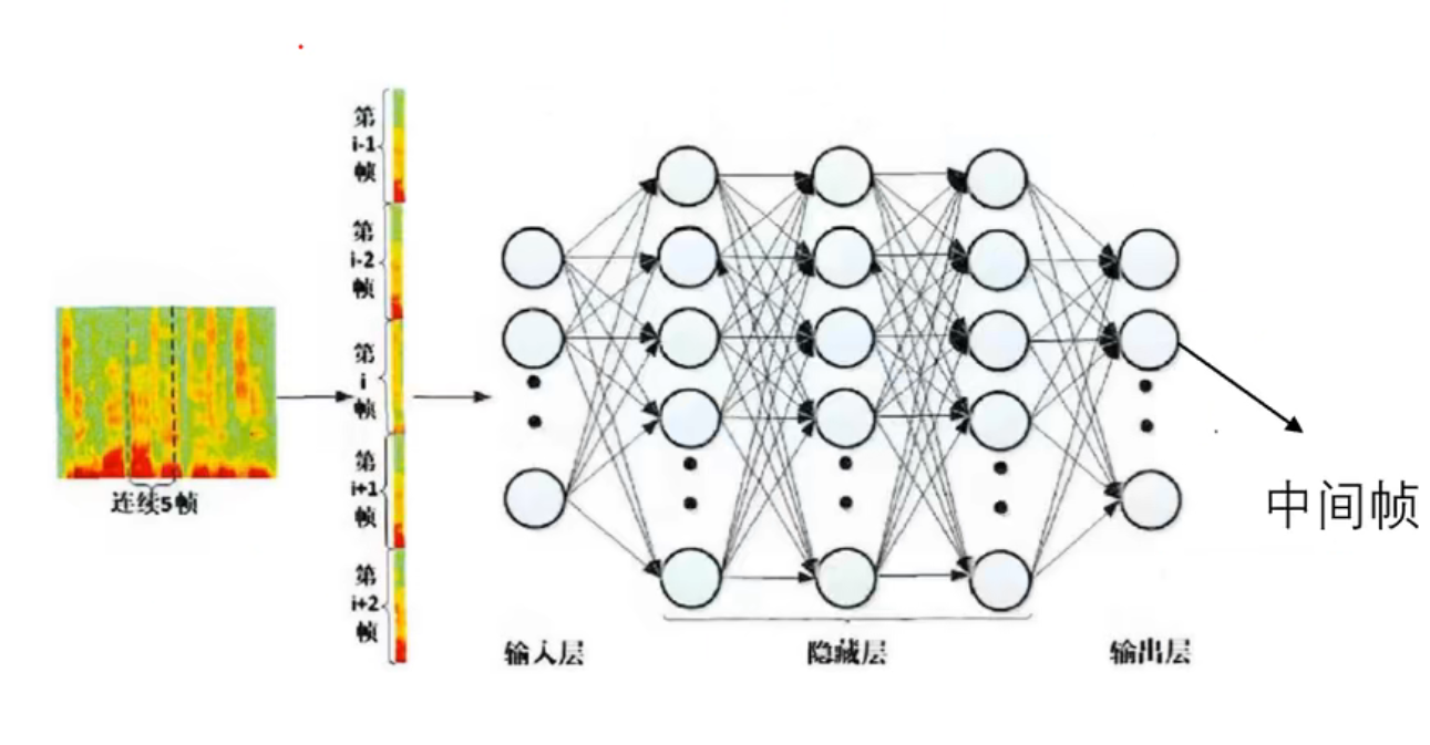
1、拼帧n_expend参数,n_expend=2),分别是第【3,4,5,6,7】帧数据,来预测(增强)第【5】帧数据,将预测得到的第5帧数据作为输出。
# dataset.py
# 数据集管理函数
import os
import torch
import numpy as np
from torch. utils. data import Dataset, DataLoader
from hparams import hparams
import librosa
import random
import soundfile as sf
# 主要用于数据管理
# 主要由 torch 中的 Dataset 与 DataLoader 类 来实现
def feature_stft ( wav, para) : # 用stft进行特征提取
spec = librosa. stft( wav,
n_fft= para[ "N_fft" ] ,
win_length = para[ "win_length" ] ,
hop_length = para[ "hop_length" ] ,
window = para[ "window" ] )
# 注意librosa.stft() 提取特征后是一个 D*T 的维度 D是特征维度=1+(nfft/2),T是帧数
mag = np. abs ( spec) # 功率模值
LPS = np. log( mag** 2 ) # 该神经网络 输入的是 幅度谱 平方后的log!!!
# Q:为什么输入的是LPS?
# A: 数据进行FFT后,幅度谱变化非常剧烈,数值不稳定,难以控制,取log以后数值稳定一些
phase = np. angle( spec) # 相位
# stft得到的是D*T 维,需要改成 T*D的格式输入, 这里的 .T 操作是转置操作
return LPS. T, phase. T # T x D
def feature_contex ( feature, expend) : # 拼帧
feature = feature. unfold( 0 , 2 * expend+ 1 , 1 ) # T x D x 2*expand+1
# 这里调用了Tensor.unfold(dimension,size,step)函数
# dimension 是沿着哪个维度重叠取帧 (T维度 ,所以是 第0维)
# size 重复取帧大小 (2*左右扩展数 +1 )
# step 步长
# 输出维度 # (T-4) x D x 2*expand+1
feature = feature. transpose( 1 , 2 ) # (T-4) x 2*n_expand+1 x D
# 把后两个维度“切换”一下
feature = feature. view( [ - 1 , ( 2 * expend+ 1 ) * feature. shape[ - 1 ] ] ) # T x (D *( 2*n_expand+1))
# 这一步,相当于保持第一维(帧 )不变,后面两维合并成了一维
return feature
class TIMIT_Dataset ( Dataset) :
def __init__ ( self, para) :
self. file_scp = para. file_scp # scp文件
self. para_stft = para. para_stft # 特征提取晚间
self. n_expand = para. n_expand # 拼帧
files = np. loadtxt( self. file_scp, dtype = 'str' ) #将噪声对scp文件读取
self. clean_files = files[ : , 1 ] . tolist( ) # 干净语音数据处于第二列
self. noisy_files = files[ : , 0 ] . tolist( ) # 含噪语音数据处于第一列
print ( len ( self. clean_files) )
print ( "干净语音第1个数据" )
print ( files[ 0 , 1 ] )
print ( "含噪语音第1个数据" )
print ( files[ 0 , 0 ] )
def __len__ ( self) : # 数据库中样本数量
return len ( self. clean_files)
def __getitem__ ( self, idx) : # 对于数据库中每一条数据的处理方法
# 读取干净语音
clean_wav, fs = sf. read( self. clean_files[ idx] , dtype = 'int16' )
clean_wav = clean_wav. astype( 'float32' )
#这里,先读取成int16格式,然后再转成float型,为什么不直接用 librosa.load()?
# 读取含噪语音
noisy_wav, fs = sf. read( self. noisy_files[ idx] , dtype = 'int16' )
noisy_wav = noisy_wav. astype( 'float32' )
# 提取stft特征
clean_LPS, _ = feature_stft( clean_wav, self. para_stft) # T x D
noisy_LPS, _= feature_stft( noisy_wav, self. para_stft) # T x D
# 转为torch格式
X_train = torch. from_numpy( noisy_LPS)
Y_train = torch. from_numpy( clean_LPS)
# 拼帧
X_train = feature_contex( X_train, self. n_expand)
Y_train = Y_train[ self. n_expand: - self. n_expand, : ]
return X_train, Y_train # 训练数据以及对应目标
def my_collect ( batch) :
# 神经网络训练时需要每一个batch大小相同
# 由于语音数据 每次训练的feasture 大小= T x (D *( 2*n_expand+1)) T帧数可能不一样 所以需要重写,实现batch的拼接
batch_X = [ item[ 0 ] for item in batch]
batch_Y = [ item[ 1 ] for item in batch]
batch_X = torch. cat( batch_X, 0 ) # 由于 T维度 可能不一样,所以沿着 T维度(第零维度)进行拼接,下同
batch_Y = torch. cat( batch_Y, 0 )
return [ batch_X. float ( ) , batch_Y. float ( ) ]
if __name__ == '__main__' :
work_path= "E:\\……\\DNN_mapping"
os. chdir( work_path)
# 数据加载测试
para = hparams( )
m_Dataset= TIMIT_Dataset( para)
m_DataLoader = DataLoader( m_Dataset, batch_size = 2 , shuffle = True , num_workers = 4 , collate_fn = my_collect)
# shuffle:随机打乱 num_workers:多线程选取 collate_fn:特征选取函数
for i_batch, sample_batch in enumerate ( m_DataLoader) : # 打印每一个batch X,Y 的特征维度
train_X = sample_batch[ 0 ]
train_Y = sample_batch[ 1 ]
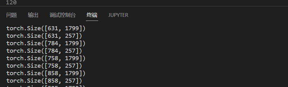
print ( train_X. shape)
print ( train_Y. shape)
torch.Size([631, 1799])
torch.Size([631, 257])
为例1799 ; 631 257
# model_mapping.py
import torch
import torch. nn as nn
from hparams import hparams
# 神经网络模型
# 采用深度神经网络
class DNN_Mapping ( nn. Module) :
def __init__ ( self, para) :
super ( DNN_Mapping, self) . __init__( )
self. dim_in = para. dim_in
self. dim_out = para. dim_out
self. dim_embeding = para. dim_embeding
self. dropout = para. dropout
self. negative_slope = para. negative_slope
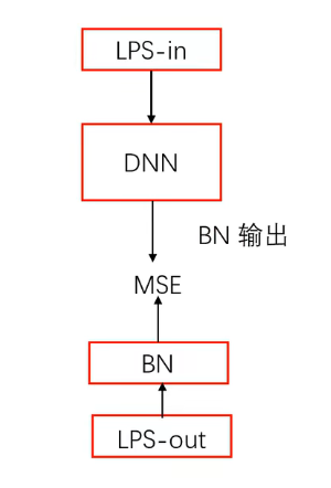
self. BNlayer = nn. BatchNorm1d( self. dim_out) # 用于归一化,语音信号经过DNN后输出再经过一个BN layer 进行输出
self. model = nn. Sequential( #DNN网络模型
# 先行正则化
nn. BatchNorm1d( self. dim_in) , #先把输入语音特征进行正则化
# 第一层
nn. Linear( self. dim_in, self. dim_embeding) ,
nn. BatchNorm1d( self. dim_embeding) ,
# nn.ReLU(),
nn. LeakyReLU( self. negative_slope) ,
nn. Dropout( self. dropout) ,
# 第二层
nn. Linear( self. dim_embeding, self. dim_embeding) ,
nn. BatchNorm1d( self. dim_embeding) ,
# nn.ReLU(),
nn. LeakyReLU( self. negative_slope) ,
nn. Dropout( self. dropout) ,
# 第三层
nn. Linear( self. dim_embeding, self. dim_embeding) ,
nn. BatchNorm1d( self. dim_embeding) ,
# nn.ReLU(),
nn. LeakyReLU( self. negative_slope) ,
nn. Dropout( self. dropout) ,
# 第四层
nn. Linear( self. dim_embeding, self. dim_out) ,
nn. BatchNorm1d( self. dim_out) ,
)
for m in self. modules( ) :
if isinstance ( m, nn. Linear) :
nn. init. xavier_normal_( m. weight. data) #神经网络Linear层初始化
def forward ( self, x, y= None , istraining = True ) :
out_enh = self. model( x)
if istraining:
out_target = self. BNlayer( y) # y 是训练目标(这里应该是纯净语音数据),也要经过一个归一化处理 BNlayer
return out_enh, out_target
else :
return out_enh
if __name__ == "__main__" :
para = hparams( )
m_model = DNN_Mapping( para)
print ( m_model)
x = torch. randn( 3 , para. dim_in)
y = m_model( x)
print ( y. shape)
# train.py
from concurrent.futures.thread import _worker
import torch
import torch.nn as nn
from hparams import hparams
from torch.utils.data import Dataset,DataLoader
from dataset import TIMIT_Dataset,my_collect
from model_mapping import DNN_Mapping
import os
# 训练过程
if __name__ == "__main__":

    # 定义device
    device = torch.device("cuda:0") # 利用gpu 进行训练,需要提前安装 cuda 以及 pytorch gpu版本

    # 获取模型参数
    para = hparams()

    # 定义模型
    m_model = DNN_Mapping(para) # 构造模型
    m_model = m_model.to(device)# 把模型的计算任务映射到gpu中计算
    m_model.train()             # 将模型置于训练模式下

    # 定义损失函数
    loss_fun = nn.MSELoss()
    # loss_fun = nn.L1Loss()
    loss_fun = loss_fun.to(device)

    # 定义优化器
    optimizer = torch.optim.Adam(
        params=m_model.parameters(),
        lr=para.learning_rate)

    # 定义数据集
    m_Dataset= TIMIT_Dataset(para)
    m_DataLoader = DataLoader(m_Dataset,batch_size = para.batch_size,shuffle = True, num_workers = 4, collate_fn = my_collect)

    # 定义训练的轮次
    n_epoch = 100 # 训练轮次,实际上7-8轮左右差不多收敛了
    n_step = 0
    loss_total = 0# 全体损失
    for epoch in range(n_epoch):
        # 遍历dataset中的数据 (通过在dataset Dataloader() 得到的 batch 的数据集)
        for i_batch, sample_batch in enumerate(m_DataLoader): # 遍历每一个batch 数据
            train_X = sample_batch[0]
            train_Y = sample_batch[1]

            train_X = train_X.to(device)
            train_Y = train_Y.to(device)

            m_model.zero_grad()
            # 得到网络输出
            output_enh,out_target = m_model(x=train_X,y=train_Y)

            # 计算损失函数
            loss = loss_fun(output_enh,out_target)

            # 误差反向传播
            # optimizer.zero_grad()
            loss.backward()

            # 进行参数更新
            # optimizer.zero_grad()
            optimizer.step()

            n_step = n_step+1
            loss_total = loss_total+loss

            # 每100 step 输出一次中间结果
            if n_step %100 == 0:
                print("epoch = %02d  step = %04d  loss = %.4f"%(epoch,n_step,loss))

        # 训练结束一个epoch 计算一次平均结果
        loss_mean = loss_total/n_step
        print("epoch = %02d mean_loss = %f"%(epoch,loss_mean))
        loss_total = 0
        n_step =0

        # 进行模型保存
        work_path="E:\\……\\DNN_mapping"
        save_path="E:\\……\\DNN_mapping\\save"
        os.chdir(work_path)
        save_name = os.path.join(save_path,'model_%d_%.4f.pth'%(epoch,loss_mean))
        torch.save(m_model,save_name)
import torch
import os
# 测试
if __name__ == "__main__" :
work_path= "E:\\homework\\……\\DNN_mapping"
os. chdir( work_path)
model_name = "save/model_4_0.0036.pth"
m_model = torch. load( model_name, map_location = torch. device( 'cpu' ) )
m_model. eval ( )
model_dic = m_model. state_dict( )
for k, v in model_dic. items( ) :
print ( 'k:' + k)
print ( v. size( ) )
print ( model_dic[ 'BNlayer.weight' ] . data)
测试函数利用 输入训练的模型 和对应参数 ,以及待增强的数据 ,具体复原操作原理 要看BatchNorm1d()函数
还原过程用到下面这个公式
y
=
x
−
E
[
x
]
Var
[
x
]
+
ϵ
∗
γ
+
β
y=\frac{x-\mathrm{E}[x]}{\sqrt{\operatorname{Var}[x]+\epsilon}} * \gamma+\beta
y = Var [ x ] + ϵ
x − E [ x ] ∗ γ + β
# eval.py
import torch
from hparams import hparams
from dataset import feature_stft, feature_contex
from model_mapping import DNN_Mapping
import os
import soundfile as sf
import numpy as np
import librosa
import matplotlib. pyplot as plt
from generate_training import signal_by_db
# 用于测试训练的模型
def eval_file_BN ( wav_file, model, para) : # 输入训练的模型和对应参数,以及待增强的数据
# 读取noisy 的音频文件
noisy_wav, fs = sf. read( wav_file, dtype = 'int16' )
noisy_wav = noisy_wav. astype( 'float32' )
# 提取LPS特征
noisy_LPS, noisy_phase = feature_stft( noisy_wav, para. para_stft)
# 转为torch格式
noisy_LPS = torch. from_numpy( noisy_LPS)
# 进行拼帧
noisy_LPS_expand = feature_contex( noisy_LPS, para. n_expand)
# 利用DNN进行增强
model. eval ( )
with torch. no_grad( ) :
enh_LPS = model( x = noisy_LPS_expand, istraining = False )
# 模型输出,注意这是一个经过BN归一化后的LPS格式输出
# 要想经模型输出 映射成正常输出,还要借助BN归一化的参数
# 具体操作原理要看BatchNorm1d()函数
# 利用 BN-layer的信息对数据进行还原
model_dic = model. state_dict( )
# gamma
BN_weight = model_dic[ 'BNlayer.weight' ] . data
BN_weight = torch. unsqueeze( BN_weight, dim = 0 )
# beta
BN_bias = model_dic[ 'BNlayer.bias' ] . data
BN_bias = torch. unsqueeze( BN_bias, dim = 0 )
# E[x]
BN_mean = model_dic[ 'BNlayer.running_mean' ] . data
BN_mean = torch. unsqueeze( BN_mean, dim = 0 )
# Var[x]
BN_var = model_dic[ 'BNlayer.running_var' ] . data
BN_var = torch. unsqueeze( BN_var, dim = 0 )
# BN反向运算,得到所求的增强信号的频谱表示(注意这里得到的依然是LPS格式,也即log)
pred_LPS = ( enh_LPS - BN_bias) * torch. sqrt( BN_var+ 1e-4 ) / ( BN_weight+ 1e-8 ) + BN_mean
# 将 LPS 还原成 Spec
pred_LPS = pred_LPS. numpy( ) # 转换成numpy格式
enh_mag = np. exp( pred_LPS. T/ 2 ) # 将log形式转换为幅度值,.T表示转置
enh_pahse = noisy_phase[ para. n_expand: - para. n_expand, : ] . T # 相位就利用原始含噪信号的相位作为增强信号的相位,但是前后扩展帧去掉
enh_spec = enh_mag* np. exp( 1j * enh_pahse) # 增强后的频谱
# istft
enh_wav = librosa. istft( enh_spec, hop_length= para. para_stft[ "hop_length" ] , win_length= para. para_stft[ "win_length" ] ) #增强后的时域信号
return enh_wav
if __name__ == "__main__" :
work_path= "E:\\……\\DNN_mapping"
os. chdir( work_path)
para = hparams( )
# 读取训练好的模型
model_name = "save/model_4_0.0036.pth"
m_model = torch. load( model_name, map_location = torch. device( 'cpu' ) )
snrs = [ 5 ]
noise_path = 'E:\\……\\NoiseX-92'
clean_path = "E:\\……\\TIMITdataset"
# noises = ['factory1','volvo','white','m109']
noises = [ 'white' ]
test_clean_files = np. loadtxt( 'scp/test_small.scp' , dtype = 'str' ) . tolist( )
path_eval = 'eval2' # 测试文件结果放在工作文件目录子文件夹 \\eval2 下
for noise in noises:
print ( noise)
noise_file = os. path. join( noise_path, noise+ '.wav' )
noise_data, fs = sf. read( noise_file, dtype = 'int16' )
for clean_wav in test_clean_files:
# 读取干净语音并保存
clean_file = os. path. join( clean_path, clean_wav)
clean_data, fs = sf. read( clean_file, dtype = 'int16' )
id = os. path. split( clean_file) [ - 1 ] # 具体文件名
sf. write( os. path. join( path_eval, id ) , clean_data, fs) #将选区的干净语音存放至eval目录下
for snr in snrs:
# 生成noisy文件
noisy_file = os. path. join( path_eval, noise+ '-' + str ( snr) + '-' + id )
mix = signal_by_db( clean_data, noise_data, snr) # 加噪声
noisy_data = np. asarray( mix, dtype= np. int16)
sf. write( noisy_file, noisy_data, fs) # 将加噪语音存储保存
# 进行增强
print ( "enhancement file %s" % ( noisy_file) )
enh_data = eval_file_BN( noisy_file, m_model, para)
# 信号正则,把信号幅度转换到±1范围内
max_ = np. max ( enh_data)
min_ = np. min ( enh_data)
enh_data = enh_data* ( 2 / ( max_ - min_) ) - ( max_+ min_) / ( max_- min_)
enh_file = os. path. join( path_eval, noise+ '-' + str ( snr) + '-' + 'enh' + '-' + id )
sf. write( enh_file, enh_data, fs) # 将增强语音保存
# 绘图
fig_name = os. path. join( path_eval, noise+ '-' + str ( snr) + '-' + id [ : - 3 ] + 'jpg' )
plt. subplot( 3 , 1 , 1 )
plt. specgram( clean_data, NFFT= 512 , Fs= fs)
plt. xlabel( "clean specgram" )
plt. subplot( 3 , 1 , 2 )
plt. specgram( noisy_data, NFFT= 512 , Fs= fs)
plt. xlabel( "noisy specgram" )
plt. subplot( 3 , 1 , 3 )
plt. specgram( enh_data, NFFT= 512 , Fs= fs)
plt. xlabel( "enhece specgram" )
plt. savefig( fig_name)