遥感+python 1.3 大气校正

2023-11-08

遥感+python 1.3 大气校正

一、大气校正概念

大气校正是指传感器最终测得的地面目标的总辐射亮度并不是地表真实反射率的反映，其中包含了由大气吸收，尤其是散射作用造成的辐射量误差。大气校正就是消除这些由大气影响所造成的辐射误差，反演地物真实的表面反射率的过程¹。
在这里插入图片描述

1、吸收和散射改变大气中的电磁辐射

从太阳到地球再回到传感器，电磁能量两次通过大气层。辐照度是来自太阳的下涌辐射。辐射是地球向传感器的上涌辐射。吸收会降低强度并产生模糊效果。散射会使大气中的电磁能重新定向，导致相邻像素共享的相邻效应。这两个过程影响图像质量，是大气校正的主要驱动力²。

2、电磁能在大气中相互作用

太阳向地球方向发射电磁能。实际上使它进入地球的电磁辐射叫做入射能量。但其中一些能量在撞击地球表面之前也会被大气中的气体和气溶胶吸收和散射。如果只有一幅图像，只有当图像非常模糊时，才需要进行大气校正。通常所有像素值都受到相同程度的影响，您可以使用所有标准分类方法获得良好的结果。大气校正去除大气中的散射和吸收效应，以获得表面反射特性（表面特性）。

二、大气校正的方法

大气校正方法可分为一下三种³：

1. 基于辐射传输方程的大气校正。

辐射传输方程具有较高的辐射校正精度，是利用电磁波在大气中的辐射传输原理建立起来的模型对遥感图像进行大气校正的方法。目前常用模型有：

6S模型
LOWTRAN（Low Resolution Transmission）
MORTRAN（Moderate Resolution Transmission）
紫外线和可见光辐射传输模型UVRAD（Ultraviolet and Visible Radiation）
空间分布快速大气校正模型ATCOR（A Spatially-Adaptive Fast AtmosphericCorrection）。

2. 基于地面场数据或辅助数据进行辐射校正。

该方法假设地面目标反射率与遥感探测器信号之间具有线性关系，并通过获取遥感影像上特定地物的灰度值及其成像时对应的地面目标反射光谱的测量值，建立两者之间的线性回归方程式，在此基础上进行对整幅遥感影像进行辐射校正。

3. 利用某些受大气影像较小的波段进行大气辐射校正。

一般情况下，散射主要发生在短波图像，对近红外几乎没有影像，如MSS-7几乎不受大气辐射的影像，把它作为无散射影像的标准图像，通过对不同波段图像的对比分析来计算大气影响。目前常用方法有：

回归分析法
暗像元法

为精度与便利性考量，本文采用6S模型。

三、大气辐射传输模型6S

6S（SecondSimulationoftheSatelliteSignalintheSolarSpectrum）模型估计了0.25-4.0μm波长电磁波在晴空无云条件下的辐射特性，是在Tanre等人提出的5S(SimulationoftheSatelliteSignalintheSolarSpectrum)基础上发展而来的。它在假设均一地表的前提下，描述了非朗伯反射地表情况下的大气影响理论，而后Vermote又将其改进为6S模型。
6S模型主要包括以下5个部分:太阳、地物与传感器之间的几何关系，大气模式，气溶胶模式，传感器的光谱特性和地表反射率，它考虑了太阳的辐射能量通过大气传递到地表，再经地表反射通过大气传递到传感器的整个传播过程。对于吸收系数的计算公式，采用了吸收线的随机指数分布统计模式，这对于宽带传感器是一种很好的近似。为了考虑多次散射及分子散射与气溶胶散射及其相互作用，6S采用最新近似(state-of-the-art)和连续散射SOS(SuccessiveOrderofScattering)方法来求解辐射传输方程。

爱学习的同学请点这里

三、代码实现

看完原理会不会很崩溃？深入浅出，从此开始(@_@)。

1、明确目的

6S模型是公开的，作为开发人员，我们简要明白其中原理即可。我们首先要明白整体的流程。

至此我们将复杂的问题逐步分解，分而治之。初看难度略大、逐一击破。

2、常规处理

2.1 获取几何参数

这种几何关系通常被保存在影像的头文件中，可以打开查看。其中通常来说，数据中保存的是太阳高程角。
太阳天顶角 = 9 0 ∘ − 太阳高程角太阳天顶角=90^{\circ}-太阳高程角太阳天顶角=90∘−太阳高程角

def getAngle(MateFile):
    SolarAzimuth = float(getInfoByMateData(MateFile, 'SolarAzimuth'))       
    SolarZenith = 90 - float(getInfoByMateData(MateFile, 'SolarZenith'))   
    SatelliteAzimuth = float(getInfoByMateData(MateFile, 'SatelliteAzimuth'))  
    SatelliteZenith = float(getInfoByMateData(MateFile, 'SatelliteZenith'))
    angle = [SolarZenith, SolarAzimuth, SatelliteZenith, SatelliteAzimuth]
    return angle

其中从XML文件中获取数据如下：

def getInfoByMateData(fileName: str, infoName):
    dom = minidom.parse(fileName)
    try:
        elements = dom.getElementsByTagName(infoName)
        element = elements[0]
        value = element.firstChild.data
        return value
    except IndexError as e:
        print(f"\033[31mcant find value by {infoName}:{e}\033[0m")
    return ""

注：在参数获取中不同人有不同的想法，在看过较多的影像参数时，我们不难发现，有许多角度值异常怪异，例如，卫星高度角在80度左右，有的又在10度左右，对于这种现象，笔者认为是由于参数含义不一致导致，于是乎有人将卫星天顶角加以判定：

	if SatelliteZenith > 45:
		SatelliteZenith = round(90 - SatelliteZenith)

2.2 获取方位信息

获取中心，即四角点坐标。同样，这些信息也被保存在头文件中。

def getExtent(MateFile):
    ul_lat = float(getInfoByMateData(MateFile, 'TopLeftLatitude'))
    ul_lon = float(getInfoByMateData(MateFile, 'TopLeftLongitude'))
    ur_lat = float(getInfoByMateData(MateFile, 'TopRightLatitude'))
    ur_lon = float(getInfoByMateData(MateFile, 'TopRightLongitude'))
    dl_lat = float(getInfoByMateData(MateFile, 'BottomLeftLatitude'))
    dl_lon = float(getInfoByMateData(MateFile, 'BottomLeftLongitude'))
    dr_lat = float(getInfoByMateData(MateFile, 'BottomRightLatitude'))
    dr_lon = float(getInfoByMateData(MateFile, 'BottomRightLongitude'))
    extent = [ul_lon, ul_lat, ur_lon, ur_lat, dl_lon, dl_lat, dr_lon, dr_lat]
    return extent

2.3 参数计算

计算高程
当然也可以利用直接写高程数据，笔者利用全球DEM数据计算影像地区的平均高程。
首先写个函数，获取影像中地理坐标的范围。

def geo2imagexy(dataset, x, y):
    '''
    根据GDAL的六 参数模型将给定的投影或地理坐标转为影像图上坐标（行列号）
    :param dataset: GDAL地理数据
    :param x: 投影或地理坐标x
    :param y: 投影或地理坐标y
    :return: 影坐标或地理坐标(x, y)对应的影像图上行列号(row, col)
    '''
    trans = dataset.GetGeoTransform()
    a = np.array([[trans[1], trans[2]], [trans[4], trans[5]]])
    b = np.array([x - trans[0], y - trans[3]])
    return np.linalg.solve(a, b)  # 使用numpy的linalg.solve进行二元一次方程的求解


def extent2xy(extent, dataset):
    xy0 = geo2imagexy(dataset, extent[0], extent[1])
    xy1 = geo2imagexy(dataset, extent[6], extent[7])
    xoffset = int(min(xy0[0], xy1[0]))
    yoffset = int(min(xy0[1], xy1[1]))
    xSize = int(max(abs(xy0[0] - xy1[0]), 1))
    ySize = int(max(abs(xy0[1] - xy1[1]), 1))
    return xoffset, yoffset, xSize, ySize

计算平均高程

def MeanDEM(extent, dem_path="Lib/GMTED2km.tif"):
    """
    计算影像所在区域的平均高程.
    """
    try:
        DEMIDataSet = gdal.Open(dem_path)
    except Exception as exception:
        print(exception)
        print(f"cannot find DEM data in file :{pathlib.Path(dem_path).resolve()}")
        return
    DEM_Band = DEMIDataSet.GetRasterBand(1)
    # 研究区矩阵行列数
    # 读取研究区内的数据，并计算高程
    xoffset, yoffset, xSize, ySize = extent2xy(extent, DEMIDataSet)
    DEMRasterData = DEM_Band.ReadAsArray(xoffset, yoffset, xSize, ySize)
    MeanAltitude = np.mean(DEMRasterData)
    return MeanAltitude

气溶胶光学厚度
气溶胶光学厚度（Aerosol Optical Depth，AOD），这一物理量被用来衡量气溶胶最基本的光学特性，它描述的是气溶胶对光的衰减作用。其定义为：气溶胶的消光系数沿着辐射传输的方向在其垂直路径上的积分。
关于气溶胶光学厚度，笔者调研了点资料，也尝试了许多方法，发现直接赋值为0.14497效果最好
计算也是可以的，其计算方法与高程相同。

def MeanAOD(extent, AOD_path):
    try:
        AODIDataSet = gdal.Open(AOD_path)
    except Exception as exception:
        print(exception)
        print(f"cannot find DEM data in file :{pathlib.Path(AOD_path).resolve()}")
        return
    AOD_Band = AODIDataSet .GetRasterBand(1)
    # 研究区矩阵行列数
    xoffset, yoffset, xSize, ySize = extent2xy(extent, AODIDataSet)
    AODRasterData = AOD_Band.ReadAsArray(xoffset, yoffset, xSize, ySize)
    MeanAODdata = np.mean(AODRasterData)
    return MeanAODdata

2.4 获取时间信息

获取时间主要是获取影像过境的中心时间，实际上差别不大。但影像参数文件中时间格式为YYYY-MM-DD HH:MM:SS，在此转化成字典模式。

def getTime(MateFile):
    time = {}
    dateTime = getInfoByMateData(MateFile, 'CenterTime')
    date, secTime = dateTime.split(" ")
    time["year"] = int(date.split("-")[0])
    time["month"] = int(date.split("-")[1])
    time["day"] = int(date.split("-")[2])
    time["hour"] = int(secTime.split(":")[0])
    time["min"] = int(secTime.split(":")[1])
    time["sec"] = int(secTime.split(":")[2])
    return time

2.5 获取波段信息

按照前文的模式从文件中读取波长信息。这里面波长信息包括：

中心波长（Central Wavelength）简称CL
波谱范围（Spectrum Range）简称SR
波谱响应函数（Spectral Response Function）简称SRF

获取示例如下，笔者只写了GF1的一个示例，可以按照这个模式接着往下写。

def getWavelengthRange(config_file, **kwargs):
    config = json.load(open(config_file))
    SatelliteID = getKwargs("SatelliteID", kwargs)
    SensorID = getKwargs("SensorID", kwargs)
    Year = getKwargs("Year", kwargs)
    ImageType = getKwargs("ImageType", kwargs)
    if SatelliteID in ["GF1"]:
        try:
            SR = config["Parameter"][SatelliteID][SensorID]["SR"]
            SR = list(SR.values())
        except KeyError:
            print(f"cannot find key {SatelliteID}-{SensorID}-SR in :{config_file}")
            SR = None
        SRF = None
        CL = None
    elif（其他类型）
    	......

2.6 大气模式判定

熟悉大气校正的同学一看就知道啦，这部分是根据纬度结合当地所在月份，设置的一个大气模式，其认为在不同月份与纬度中，存在不同的大气廓线，对电磁波存在不同的影响。

无气体吸收
热带大气
中纬度夏大气
中纬度冬季
亚北极区夏季
亚北极区冬季
美国标准大气（62年）
用户定义大气廓线（34层无线电探空数据）包括：高度（km）气压( mb )温度( k )水汽密度(g/m3)臭氧密度(g/m3)
输入水汽和臭氧总含量水汽( g/cm2)臭氧(cm-atm)
读入无线电探空数据文件

def getPredefinedType(lat, month):
    predefinedType = None
    if -15 < lat < 15:
        predefinedType = AtmosProfile.PredefinedType(AtmosProfile.Tropical)
    if 15 < lat < 45:
        if 4 < month < 9:
            predefinedType = AtmosProfile.PredefinedType(AtmosProfile.MidlatitudeSummer)
        else:
            predefinedType = AtmosProfile.PredefinedType(AtmosProfile.MidlatitudeWinter)
    if 45 < lat < 60:
        if 4 < month < 9:
            predefinedType = AtmosProfile.PredefinedType(AtmosProfile.SubarcticSummer)
        else:
            predefinedType = AtmosProfile.PredefinedType(AtmosProfile.SubarcticWinter)
    return predefinedType

2.7 6S模型参数获取

就按照上流程图所示，将各个参数输入到6S模型当中。（参考文献）

def AtmosphericCorrection_parameter(angle, date, latlon, dem, aod, **kwargs):
	#6s.exe默认路径
    SixS_PATH = getKwargs("SixS_PATH", kwargs, default=config.SixS_PATH)
    #获取波段信息
    SpectrumRange = getKwargs("SpectrumRange", kwargs, default=None, debug=False)
    SpectrumRangeFunction = getKwargs("SpectrumRangeFunction", kwargs, default=None, debug=False)
    CentralWavelength = getKwargs("CentralWavelength", kwargs, default=None, debug=False)
    # 6S模型
    s = SixS(SixS_PATH)
    # 传感器类型 自定义
    s.geometry = Geometry.User()
    # 太阳天顶角 太阳方位角,观测天顶角，观测方位角，日期
    s.geometry.solar_z = angle[0]
    s.geometry.solar_a = angle[1]
    s.geometry.view_z = 0
    s.geometry.view_a = 0
    s.geometry.month = date["month"]
    s.geometry.day = date["day"]
    lat = latlon[1]
    # 大气模式类型 根据经度判断
    s.atmos_profile = getPredefinedType(lat, date["month"])

    # 气溶胶类型 大陆气溶胶 后续可以继续根据其他元素进行判断。
    s.aero_profile = AtmosProfile.PredefinedType(AeroProfile.Continental)
    # 下垫面类型
    s.ground_reflectance = GroundReflectance.HomogeneousLambertian(0.36)

    # 550nm气溶胶光学厚度,对应能见度为40km  可以更精细
    s.aot550 = aod

    # 研究区海拔、卫星传感器轨道高度
    s.altitudes = Altitudes()
    s.altitudes.set_target_custom_altitude(dem)  # dem获取,从其他函数中获取
    s.altitudes.set_sensor_satellite_level()

    # 校正波段（根据波段名称）
    if SpectrumRangeFunction is not None:
        s.wavelength = Wavelength(SpectrumRange[0], SpectrumRange[1], SpectrumRangeFunction)
    elif SpectrumRange is not None:
        s.wavelength = Wavelength(SpectrumRange[0], SpectrumRange[1])
    else:
        s.wavelength = Wavelength(CentralWavelength)
    # 下垫面非均一、朗伯体
    s.atmos_corr = AtmosCorr.AtmosCorrLambertianFromReflectance(-0.1)  # 此处使用朗伯体，不考虑下垫面非均一，即不考虑BRDF
    # 运行6s大气模型
    s.run()  # 消耗时间过大
    xa = s.outputs.coef_xa
    xb = s.outputs.coef_xb
    xc = s.outputs.coef_xc
    out = (xa, xb, xc)
    return out

在此大家可以打开调试模式，查看s.outputs中都含有什么参数，基本上你想要的都有，有惊喜&_&。

注：有不理解的吗？有！为什么观测天顶角，观测方位角归零了？不理解。前文此参数已经获取到了，但此处没有用，大家可以用获取到的参数输入进去试一试，笔者在尝试过程中，其结果并不理想，而默认为0，曲线很好看，神奇！

2.7 反射率计算

在此获取了xa, xb, xc，基本上大功告成。
下面利用公式。
ρ = y 1 + y ∗ c y = a ∗ L − b \rho=\dfrac{y}{1+y*c}\\ y=a*L-b ρ=1+y∗cyy=a∗L−b

    for i_bandNo in range(0, bandCount):
        a = aList[i_bandNo]
        b = bList[i_bandNo]
        c = cList[i_bandNo]
        Image_block_band = inDataset.GetRasterBand(i_bandNo + 1).ReadAsArray(xoffset, yoffset, nXblock, nYblock)
        if isRadiometric is False:
            Image_block_band = Image_block_band * gain[i_bandNo] + offset[i_bandNo]
        y = a * Image_block_band - b
        Image_block_band = (y / (1 + y * c)) * 10000
        Image_block_band[~Image_block_full] = 0
        Image_block_band = Image_block_band.astype(np.uint16)
        outband = outDataset.GetRasterBand(i_bandNo + 1)
        outband.WriteArray(Image_block_band, xoffset, yoffset)

3、分块处理

若影像覆盖面积较大，影像各部分区域差别较为明显，为提高精度，采取影像分块计算模式。

3.1 获取几何参数

由于距离原因，太阳角度几乎不变，而观测角度会产生较大变化。
在此可以采用克里金插值。

        lin_middle = im_height / 2.0
        sam_middle = im_width / 2.0
        sam = [sam_TopLeft, sam_TopRight, sam_BotRight, sam_BotLeft, sam_middle]  # （经度）左上、右上、右下、左下
        lin = [lin_TopLeft, lin_TopRight, lin_BotRight, lin_BotLeft, lin_middle]  # （纬度）左上、右上、右下、左下
        if wfv_flag == 'WFV1' or wfv_flag == 'WFV2':
            # zenith = [100*(SatelliteZenith + 9), 100*(SatelliteZenith - 9), 100*(SatelliteZenith - 9), 100*(SatelliteZenith + 9), round(100*SatelliteZenith,4)]
            zenith = [(SatelliteZenith + 9), (SatelliteZenith - 9), (SatelliteZenith - 9), (SatelliteZenith + 9),
                      round(SatelliteZenith, 4)]
        else:
            # zenith = [100*(SatelliteZenith - 9), 100*(SatelliteZenith + 9), 100*(SatelliteZenith + 9), 100*(SatelliteZenith - 9), round(100*SatelliteZenith,4)]
            zenith = [(SatelliteZenith - 9), (SatelliteZenith + 9), (SatelliteZenith + 9), (SatelliteZenith - 9),
                      round(SatelliteZenith, 4)]
        pi = 3.14159
        vz = kriging(sam, lin, zenith, im_width, im_height)

或者利用scipy.interpolate.interp2d双线性插值。

3.2 获取方位信息

将影像切块，获取每一块的中心经纬度。结果为h列w行，经纬（h*w*【经度，纬度】）

def getCentreMap(extent, row_Number, col_Number):
    # 控制经度
    X_lonIndex_list = np.asarray([0, 1])
    Y_lonIndex_list = np.asarray([0, 1])
    X_lonIndex_Map, Y_lonIndex_Map = np.meshgrid(X_lonIndex_list, Y_lonIndex_list)
    lonIndex_Map = np.zeros(X_lonIndex_Map.shape)
    lonIndex_Map[0, 0] = extent[0]
    lonIndex_Map[0, 1] = extent[2]
    lonIndex_Map[1, 0] = extent[4]
    lonIndex_Map[1, 1] = extent[6]
    lonInterp2d = interp2d(X_lonIndex_list, Y_lonIndex_list, lonIndex_Map, kind='linear')
    X_lonIndexlist = np.linspace(0, 1, col_Number * 2 + 1)
    Y_lonIndexlist = np.linspace(0, 1, row_Number * 2 + 1)
    lonIndexMap = lonInterp2d(X_lonIndexlist, Y_lonIndexlist)
    # 控制纬度
    X_latIndex_list = np.asarray([0, 1])
    Y_latIndex_list = np.asarray([0, 1])
    X_latIndex_Map, Y_latIndex_Map = np.meshgrid(X_latIndex_list, Y_latIndex_list)
    latIndex_Map = np.zeros(X_latIndex_Map.shape)
    latIndex_Map[0, 0] = extent[1]
    latIndex_Map[0, 1] = extent[3]
    latIndex_Map[1, 0] = extent[5]
    latIndex_Map[1, 1] = extent[7]
    latInterp2d = interp2d(X_latIndex_list, Y_latIndex_list, latIndex_Map, kind='linear')
    X_latIndexlist = np.linspace(0, 1, col_Number * 2 + 1)
    Y_latIndexlist = np.linspace(0, 1, row_Number * 2 + 1)
    latIndexMap = latInterp2d(X_latIndexlist, Y_latIndexlist)
    centrePointMap = np.zeros((row_Number, col_Number, 2))
    for height_i in range(1, row_Number * 2 + 1, 2):
        height_o = int((height_i + 1) / 2) - 1
        for width_i in range(1, col_Number * 2 + 1, 2):
            width_o = int((width_i + 1) / 2) - 1
            centrePointMap[height_o, width_o, 0] = lonIndexMap[height_i, width_i]
            centrePointMap[height_o, width_o, 1] = latIndexMap[height_i, width_i]
    return centrePointMap

同理计算影像范围，为DEM计算，AOD计算做铺垫。结果为h列w行+8维数据（h*w*2），其中8维数据为
0.左上点经度，
1.左上点纬度，
2.右上点经度，
3.右上点纬度，
4.左下点经度，
5.左下点纬度，
6.右下点经度，
7.右下点纬度。

def getExtentMap(extent, row_Number, col_Number):
    # 控制经度
    X_lonIndex_list = np.asarray([0, 1])
    Y_lonIndex_list = np.asarray([0, 1])
    X_lonIndex_Map, Y_lonIndex_Map = np.meshgrid(X_lonIndex_list, Y_lonIndex_list)
    lonIndex_Map = np.zeros(X_lonIndex_Map.shape)
    lonIndex_Map[0, 0] = extent[0]
    lonIndex_Map[0, 1] = extent[2]
    lonIndex_Map[1, 0] = extent[4]
    lonIndex_Map[1, 1] = extent[6]
    lonInterp2d = interp2d(X_lonIndex_list, Y_lonIndex_list, lonIndex_Map, kind='linear')
    X_lonIndexlist = np.linspace(0, 1, col_Number * 2 + 1)
    Y_lonIndexlist = np.linspace(0, 1, row_Number * 2 + 1)
    lonIndexMap = lonInterp2d(X_lonIndexlist, Y_lonIndexlist)
    # 控制纬度
    X_latIndex_list = np.asarray([0, 1])
    Y_latIndex_list = np.asarray([0, 1])
    X_latIndex_Map, Y_latIndex_Map = np.meshgrid(X_latIndex_list, Y_latIndex_list)
    latIndex_Map = np.zeros(X_latIndex_Map.shape)
    latIndex_Map[0, 0] = extent[1]
    latIndex_Map[0, 1] = extent[3]
    latIndex_Map[1, 0] = extent[5]
    latIndex_Map[1, 1] = extent[7]
    latInterp2d = interp2d(X_latIndex_list, Y_latIndex_list, latIndex_Map, kind='linear')
    X_latIndexlist = np.linspace(0, 1, col_Number * 2 + 1)
    Y_latIndexlist = np.linspace(0, 1, row_Number * 2 + 1)
    latIndexMap = latInterp2d(X_latIndexlist, Y_latIndexlist)
    ExtentMap = np.zeros((row_Number, col_Number, 8))
    for height_i in range(1, row_Number * 2 + 1, 2):
        height_o = int((height_i + 1) / 2) - 1
        for width_i in range(1, col_Number * 2 + 1, 2):
            width_o = int((width_i + 1) / 2) - 1
            # print(height_o,width_o)
            ExtentMap[height_o, width_o, 0] = lonIndexMap[height_i - 1, width_i - 1]
            ExtentMap[height_o, width_o, 1] = latIndexMap[height_i - 1, width_i - 1]
            ExtentMap[height_o, width_o, 2] = lonIndexMap[height_i - 1, width_i + 1]
            ExtentMap[height_o, width_o, 3] = latIndexMap[height_i - 1, width_i + 1]
            ExtentMap[height_o, width_o, 4] = lonIndexMap[height_i + 1, width_i - 1]
            ExtentMap[height_o, width_o, 5] = latIndexMap[height_i + 1, width_i - 1]
            ExtentMap[height_o, width_o, 6] = lonIndexMap[height_i + 1, width_i + 1]
            ExtentMap[height_o, width_o, 7] = latIndexMap[height_i + 1, width_i + 1]
    return ExtentMap

当然，这种插值计算的方法精度未必做好，但勉强可以使用，还可以利用空间计算的方式，将其角度计算出来，但这种计算涉及到空间球体坐标计算角度，再切换一下坐标系，我并不会T_T。

四、代码疑问

1、路径错误

错误提示：
UnicodeDecodeError: 'utf-8' codec can't decode byte 0xb2 in position 44: invalid start byte
路径错误提示
解决方法：检查路径中是否有中文（或者中文标点），再检查一下路径是否准确无误。这个基本上就是未找到6s.exe。

2、参数文件读取错误

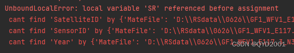
错误提示：
UnboundLocalError: local variable 'SR' referenced before assignment
参数文件读取错误提示
解决方法：检查getInfoFromFilename是否可以处理您输入的影像命名规范，可以修改其规范达到您所处理的目标影像。

def getInfoFromFilename(filename: str, type=None):
    infoDict = {}
    infoList = filename.split("_")
    if type is None:
        type = infoList[0]
    if type in ["GF1", "GF1B", "GF1C", "GF1D"]:
        infoDict["SatelliteID"] = infoList[0]
        infoDict["SensorID"] = infoList[1]
        infoDict["Year"] = infoList[4][:4]
        try:
            ImageTypeStr = infoList[5].split("-")[1]
            infoDict["ImageType"] = ImageTypeStr
        except Exception as e:
            print(f"cannot find ImageType in {filename}")
    elif type in ["GF2"]:
        infoDict["SatelliteID"] = infoList[0]
        infoDict["SensorID"] = infoList[1]
        infoDict["Year"] = infoList[4][:4]
        ImageTypeStr = infoList[5].split("-")[1]
        infoDict["ImageType"] = ImageTypeStr

若函数RadiometricCalibration出现相同错误，采用同样修改方法。

<返回目录

张安定．遥感原理与应用题解：科学出版社，2016 ↩︎
什么是遥感中的大气校正？ ↩︎
光学卫星遥感影像大气校正的方法 ↩︎

本文内容由网友自发贡献，版权归原作者所有，本站不承担相应法律责任。如您发现有涉嫌抄袭侵权的内容，请联系:hwhale#tublm.com(使用前将#替换为@)