logistic regression
一、Logistic 回归(利用matlib实现:基础版)
1、logistic regression数学基础
1.1 此示例为二元分类,二元分类的最终预测结果h为{0, 1},为获得此效果,使用sigmoid函数/logistic函数:
g
(
z
)
=
1
/
1
+
e
x
p
(
−
z
)
g(z) = 1 / 1 + exp(-z)
g(z)=1/1+exp(−z)
效果图如下:

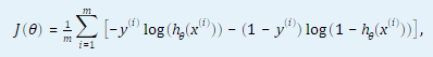
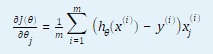
1.2 计算代价函数和代价函数对θ(j) (j = 0, …,n,n为特征数量)的偏导数。
2. 代码分析
2.1 对数据进行预处理,获得特征矩阵X,和答案向量y;
data = load('ex2data1.txt');
[m, n] = size(data);
X = data(:,1:2);
X = [ones(m,1), X];
y = data(:,3);
2.2 将数据分为正样本,负样本,并进行可视化, plotData(X, y).m;
function plotData(X, y)
figure; hold on;
pos = find(y);
neg = find(y == 0);
plot(X(pos,1), X(pos, 2), 'k+','LineWidth', 2, 'MarkerSize', 7);
plot(X(neg,1), X(neg, 2), 'ko', 'MarkerFaceColor', 'y','MarkerSize', 7);

end
2.3 初始化训练参数theta
initial_theta = zeros(n,1);
2.4 计算初始化的cost 和 grad,定义函数costFunction(initial_theta, X, y)
function [J, grad] = costFunction(theta, X, y)
m = length(y); % number of training examples
J = 0;
grad = zeros(size(theta));

h = sigmoid(X * theta);
J = -sum(y .* log(h) + (1-y) .* log(1-h))/m;

error = h - y;
grad = (X' * error)/m;

end
2.5 使用fminunc得到优化的theta和对应的cost:fminunc()函数会自动计算出合适的theta,并求出对应的cost,只需输入初始化theta,并且无需编写theta = theta - gradient,只需在fminunc@的函数中写出J 和 gradient
% 设置fminunc的选项
options = optimoptions(@fminunc, 'Algorithm', 'Quasi-Newton', 'GradObj', 'on', 'MaxIter',400);

% 运行fminunc获得最优的theta
% 这个方程将会返回theta和cost
[theta, cost] = fminunc(@(t)costFunction(t,X,y), initial_theta, options);
2.6 画出决策边界;定义函数plotDecisionBoundary(theta,X,y);
function plotDecisionBoundary(theta, X, y)

plotData(X(:,2:3), y);
hold on

if size(X, 2) <= 3
    plot_x = [min(X(:,2))-2,  max(X(:,2))+2];

    plot_y = (-1./theta(3)).*(theta(2).*plot_x + theta(1));

    plot(plot_x, plot_y)

    legend('Admitted', 'Not admitted', 'Decision Boundary')
    axis([30, 100, 30, 100])
else

    u = linspace(-1, 1.5, 50);
    v = linspace(-1, 1.5, 50);

    z = zeros(length(u), length(v));

    for i = 1:length(u)
        for j = 1:length(v)
            z(i,j) = mapFeature(u(i), v(j))*theta;
        end
    end
    z = z'; % important to transpose z before calling contour

    contour(u, v, z, [0, 0], 'LineWidth', 2)
end
hold off

end
2.7 输入新样本进行预测
prob = sigmoid([1 45 85] * theta);
2.8 计算训练集的准确度;定义函数predict(theta, X);
function p = predict(theta, X)

m = size(X, 1); % Number of training examples
p = zeros(m, 1);
s = sigmoid(X * theta);
p = s >= 0.5;

end
整体代码如下:
clear all; close all; clc
% 获取数据并构建特征值矩阵X, 结果向量y
data = load('ex2data1.txt');
[m, n] = size(data);
X = data(:,1:2);
X = [ones(m,1), X];
y = data(:,3);

% 数据可视化
plotData(X,y);

%定义轴标签
xlabel('Exam 1 score')
ylabel('Exam 2 score')

%显示图例
legend('Admitted', 'Not admitted')

%初始化训练参数
initial_theta = zeros(n,1);

%计算并打印初始cost和gradient
[cost, grad] = costFunction(initial_theta,X,y);
fprintf('Cost at initial theta(zeros): %f\n', cost);
disp('Gradient at initial theta:'); disp(grad);

% 设置fminunc的选项
options = optimoptions(@fminunc, 'Algorithm', 'Quasi-Newton', 'GradObj', 'on', 'MaxIter',400);

% 运行fminunc获得最优的theta
% 这个方程将会返回theta和cost
[theta, cost] = fminunc(@(t)costFunction(t,X,y), initial_theta, options);

% 显示theta
fprintf('Cost of theta found by fminunc: %f\n', cost);
disp('theta:'); disp(theta);

% 数据可视化
plotDecisionBoundary(theta,X,y);

%定义轴标签
xlabel('Exam 1 score')
ylabel('Exam 2 score')

%显示图例
legend('Admitted', 'Not admitted')
hold off;

%预测一个学生第一次考试为45,第二次考试为85,通过的可能性。
prob = sigmoid([1 45 85] * theta);
fprintf('For a student with scores 45 and 85, we predict an admission probability of %f\n\n', prob);
%计算训练集的准确度
p = predict(theta, X);
fprintf('Train Accuracy: %f\n', mean(double(p == y)) * 100);
结果图如下:

二、Logistic 回归(利用matlib实现:进阶版)
1.基本思想
使用fitglm函数获得logistic regression模型来预测通过的可能性。
2. 代码分析
2.0 本地函数:plotMdlData函数
plotMdlData用于绘制数据集的正例和负例,以便更好地与ex2中的图进行比较。
function [] = plotMdlData(data)
% Reproduce the plots from ex2 with positive and negative results for an input table
% Extract variable names from 3 column table
varNames = data.Properties.VariableNames;
% Plot the data with + for true and 0 for false examples
inds = data.(varNames{3}) == 1;
plot(data.(varNames{1})(inds), data.(varNames{2})(inds), 'k+','LineWidth', 2, 'MarkerSize', 7);
inds = data.(varNames{3}) == 0;
plot(data.(varNames{1})(inds), data.(varNames{2})(inds), 'ko', 'MarkerFaceColor', 'y','MarkerSize', 7);
end
2.1 将数据加载为一个表,并预览数据
clear:
data = readtable('ex2data1.txt');
data.Properties.VariableNames = {'Exam1', 'Exam2', 'Admitted'};
data.Admitted = logical(data.Admitted)
% 显示数据表总体信息
summary(data)
结果如下:

2.2 使用fitglm训练模型
Logistic回归模型属于一类较大的线性模型,在MATLAB中被称为广义线性模型。 为了训练广义线性模型,我们使用fitglm函数。 运行本节中的代码以在exam data 上训练逻辑回归模型。 结果是GeneralizedLinearModel变量,其中包含有关模型的所有信息。 请注意,要从fitglm获得logistic回归模型,我们将Distribution参数设置为二项式,如以下代码所示:
logMdl = fitglm(data,'Distribution','binomial')
结果如下:

注意上面输出中显示的模型形式。 这是对以下公式的简写:
l
o
g
i
t
(
A
d
m
i
t
t
e
d
)
=
1
∗
θ
0
+
E
x
a
m
1
∗
θ
1
+
E
x
a
m
2
∗
θ
2
logit(Admitted) = 1 * θ0 + Exam1 * θ1 + Exam2 * θ2
logit(Admitted)=1∗θ0+Exam1∗θ1+Exam2∗θ2
由于是 sigmoid(x) 的反函数,因此该模型等效于由用ex2中的Admitted概率组成的logistic回归模型:

其中包括两个考试成绩和一个偏差项。 与fitlm在ex1脚本中训练的线性回归模型一样,fitglm自动添加偏差项。
2.3 预测训练准确率和通过的可能性
theta = logMdl.Coefficients.Estimate
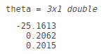
% Predict the probability for a student with scores of 45 and 85
prob = predict(logMdl,[45 85]);
fprintf('For a student with scores 45 and 85, we predict an admission probability of %f\n\n', prob);
% Compute the training accuracy
Admitted = predict(logMdl,data) > 0.5;
fprintf('Train Accuracy: %f\n', mean(double(Admitted == data.Admitted)) * 100);
2.4 可视化决策边界
figure; hold on;
% Plot the positive and negative examples
plotMdlData(data);

% Plot the decision boundary
xvals = [min(data.Exam1), max(data.Exam1)];
yvals = -(theta(1)+theta(2)*xvals)/theta(3);
plot(xvals,yvals); hold off;
ylim([min(data.Exam2),max(data.Exam2)]);

% Labels and Legend
xlabel('Exam 1 score')
ylabel('Exam 2 score')
legend('Admitted','Not admitted','Decision Boundary')
hold off;

三、正则化regularized logistic 回归
1.基本思想:
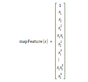
1.1 更好地拟合数据的一种方法是从每个数据点创建更多特征。
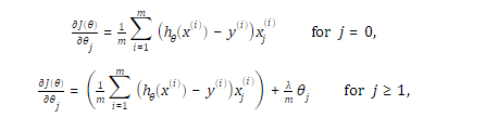
1.2 修改代价函数和梯度为:

2.代码分析:
2.1 增加多项式特征:定义mapFeature(X1, X2)函数
X = mapFeature(X(:,1),X(:,2));
function out = mapFeature(X1, X2)
degree = 6;
out = ones(size(X1(:,1)));
for i = 1:degree
    for j = 0:i
        out(:, end+1) = (X1.^(i-j)).*(X2.^j);
    end
end

end
2.2 计算正则化logistic回归的cost和grad:定义costFunctionReg(theta, X, y)
function [J, grad] = costFunctionReg(theta, X, y, lambda)
m = length(y); % number of training examples

J = 0;
grad = zeros(size(theta));

h = sigmoid(X * theta);
reg = (lambda / (2*m)) * sum(theta(2:end) .^ 2);
J = -1/m * sum(y .* log(h) + (1-y) .* log(1-h)) + reg;

error = h - y;
tmp = theta;
tmp(1) = 0;
grad = (1/m) * (X' * error) + lambda/m*tmp;
完整代码:
clear all; close all; clc
% 初始化数据,特征值矩阵,结果向量
data = load('ex2data2.txt');
X = data(:,1:2);
y = data(:,3);

%可视化数据
plotData(X, y)
xlabel('Microchip test 1')
ylabel('Microchip test 2')
legend('y = 1', 'y = 0')

%增加多项式特征
X = mapFeature(X(:,1),X(:,2));
[m, n] = size(X);

%初始化theta,lambda
initial_theta = zeros(n,1);
lambda = 1;

%计算和显示初始化的theta的cost和grad
[cost, grad] = costFunctionReg(initial_theta, X, y, lambda)
fprintf('cost at initial theta (zeros): %f\n', cost);
disp('grad:'); disp(grad);

%运行fminunc获得最优theta,无需指定学习率和循环
%返回theta和cost
options = optimoptions(@fminunc, 'Algorithm', 'Quasi-Newton', 'GradObj', 'on', 'MAXITER', 1000);

[theta, J, exit_flag] = fminunc(@(t)costFunctionReg(t,X,y,lambda), initial_theta, options);

%显示theta和J
fprintf('cost at  theta found by fminuc: %f\n',J);
disp('theta: '); disp(theta);

%可视化决策边界
plotDecisionBoundary(theta ,X, y)
xlabel('Microchip test 1')
ylabel('Microchip test 2')

legend('y = 1', 'y = 0', 'Decision boundary')
hold off;

% 计算训练集的准确率
p = predict(theta, X);

fprintf('Train Accuracy: %f\n', mean(double(p == y)) * 100);
结果图如下:

四、正则化regularized logistic 回归(进阶版)
1、基本思想:
我们使用fitclinear函数训练一个包括正则化的逻辑回归模型。 由于fitclinear函数通常用于高维数据(即具有很多变量,例如我们的多项式特征模型),因此在表变量中存储数据的意义不大,因此取而代之的是采用数字矩阵形式的训练数据。
2、代码分析:
2.1 加载数据
clear;
X = load('ex2data2.txt');
y = X(:,3);
X(:,3) = [];
% Create the polynomial feature matrix up to power 6
powers = [nchoosek(0:6,2); fliplr(nchoosek(0:6,2));1 1;2 2;3 3]';
powers(:,sum(powers)>6) = [];
Xpoly = (X(:,1).^powers(1,:)).*(X(:,2).^powers(2,:));
2.2 训练模型
我们使用fitclinear训练模型,并将正则化类型设置为ridge(这是ex2中使用的正则化类型),并使用lambda给出强度。 结果是一个ClassificationLinear模型变量,其中包含有关模型的所有信息。 在模型变量的Bias和Beta属性中可以找到模型系数。 使用控件选择一个值,然后从以下两个部分的结果中检查对训练准确性和决策边界的影响:
% Choose lambda and train the model
lambda = 0.001;
logMdl = fitclinear(Xpoly,y,'Lambda',lambda,'Learner','logistic','Regularization','ridge')
logMdl.Bias
logMdl.Beta
2.3 使用正则化模型预测类并绘制决策边界
将预测函数用于使用CategoryLinear模型变量以与GeneralizedLinearModel变量相同的方式对数据进行分类。 但是,预测函数将返回类标签,而不是概率得分。 如果需要,我们可以通过请求预测的第二个输出来获得概率分数。
% Obtain the class labels and compute the training accuracy
Pass = predict(logMdl,Xpoly);
fprintf('Train Accuracy: %f\n', mean(Pass == y) * 100);
% Plot the positve and negative examples
figure; hold on;
plotMdlData(array2table([X y],'VariableNames',{'Test1','Test2','Pass'}));

% Plot the decision boundary
xvals = linspace(min(X(:,1)), max(X(:,1)));
yvals = linspace(min(X(:,2)), max(X(:,2)));
[Xgrid, Ygrid] = meshgrid(xvals,yvals);
Xpolygrid = (Xgrid(:).^powers(1,:)).*(Ygrid(:).^powers(2,:));
[~,Score] = predict(logMdl,Xpolygrid); % Obtain the probability scores
contour(Xgrid,Ygrid,reshape(Score(:,2),size(Xgrid)),[0.5,0.5]); hold off;
% Labels and legend
xlabel('Test 1 score')
ylabel('Test 2 score')
legend('Pass', 'Fail','Decision Boundary')
以上为matlib实现logistic regression,在下面这边文档中将使用Python实现该分类算法。