论文:Grounded Language-Image Pre-training
代码:https://github.com/microsoft/GLIP
出处:微软 | 华盛顿大学
时间:2022.06
效果:
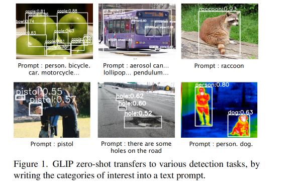
视觉识别模型一般都使用提前设定的类别来进行训练,这会限制器在真实场景中的使用
CLIP 方法证明了 image-level 的视觉特征表达能够很好的学习大量的 image-text pairs
其 text 中包含很丰富的视觉概念,pre-trained CLIP 模型语义非常丰富,能够很好的泛化到下游的 zero-shot 图像分类、图文检索
为了更细粒度的对图像理解,目标检测、分割、姿态估计、场景理解等 object-level 的任务也非常重要。
本文的重点:
相关工作:
标准的目标检测系统一般是在特定的标注类别数据上进行训练,如 COCO [37], OpenImages (OI) [30], Objects365 [50], and Visual Genome (VG),这些数据集的类别不超过 2000 类。
CLIP 和 ALIGN 这些方法的出现将图文对比学习带入大众的视野,证明了能够利用大量的图文对儿来实现开放词汇的图像分类
之后就有 ViLD 方法将 CLIP 学习到的知识蒸馏到两阶段检测器上来实现开放词汇的目标检测,还有 MDETR 方法训练了一个端到端的目标检测器来将 phrase 和 object 进行对齐
GLIP 是承接 MDETR 这条线的,主要聚焦于不同域之间的迁移,希望能做到一个预训练模型迁移到很多下游任务和领域中
zero-shot 目标检测的方法:
GLIP 和 zero-shot 目标检测的不同:
很多开放世界目标检测的方法将[能够检测出任何新类目标]作为一个挑战点,而 GLIP 是在具有检出所有可能类别的前提下检出 prompt 提及的类别即可
同时 GLIP 也会考虑迁移到使用场景的花费,比如如何使用很少的数据、训练时间、硬件机器等的同时还能获得很好的效果
所以,GLIP 支持 prompt tuning,因为 GLIP 发现 prompt tuning 能够在达到 full tine-tuning 的效果的同时,只需要调整很少的参数
且 GLIP 发现在目标检测中,prompt tuning 更适合于 vision-language deep fusion 的模型(GLIP),这也推翻了之前的证明说 prompt tuning 只适合与 shallow-fused vision-language 模型(如 CLIP)
GLIP 主要内容如下:
1、将 object detection 任务重建为 phrase grounding
如何重建任务:
detection 和 grounding 任务统一有什么好处:能够同时利用两个任务的数据并且互利互惠
2、使用大量的 image-text data 扩充视觉概念
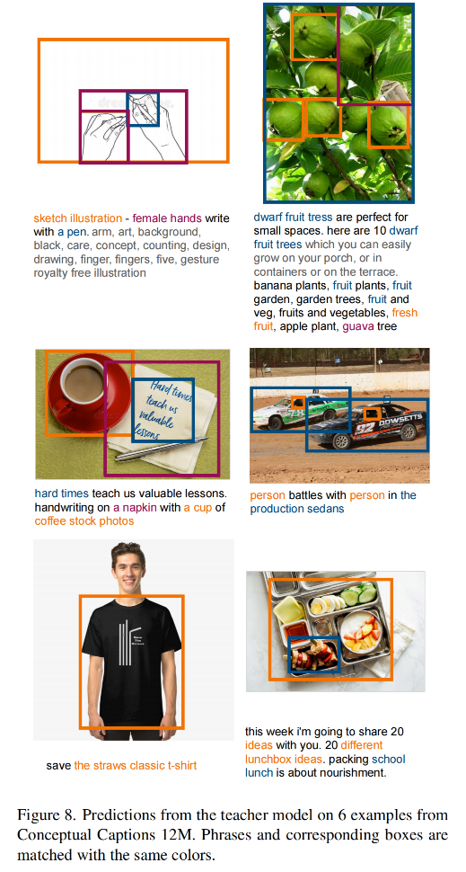
假设有一个很好的 grounding model(teacher),则可以为这些大量的 image-text-paired 数据自动生成 grounding box ,phrase 可以使用 NLP parser 来检测
teacher model 能对一些难定论的目标或抽象的目标进行定位,也能带来很丰富的语义信息
所以,可以在 27M grounding data 上 pre-train 我们的 student GLIP-large model(GLIP-L)
27M grounding data :
3、使用 GLIP 进行迁移学习:从一个 model 到所有 model
当 GLIP-L 模型在 COCO 和 LVIS 数据集上直接进行验证(没有见过其他数据),就能在 COCO val 2017 上达到 49.8 AP,在 LVIS val 上达到 26.9 AP ,超越了很多基础方法
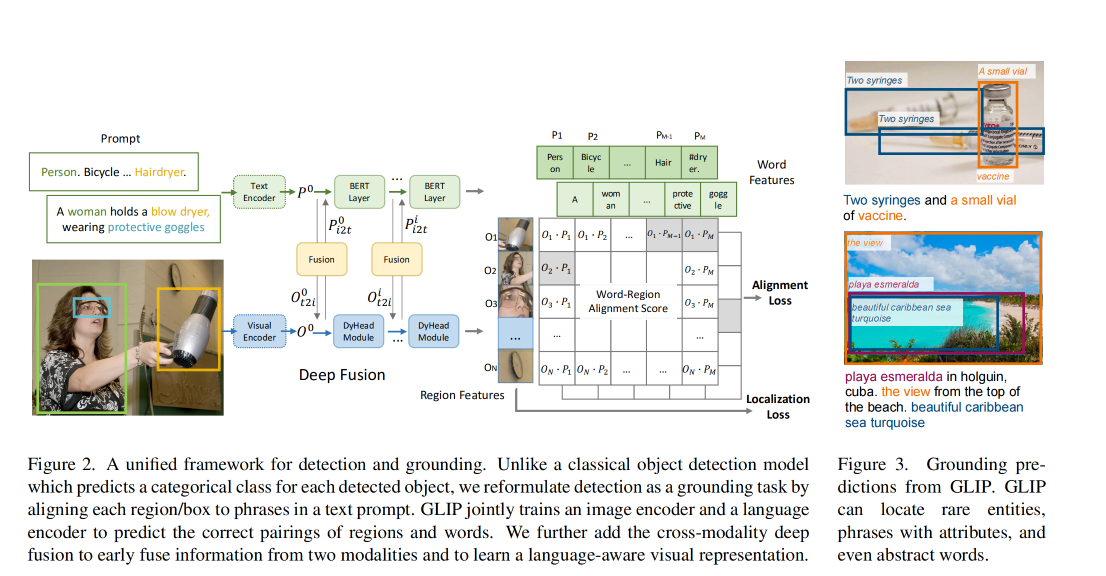
1、传统的目标检测任务:
是将图像输入 backbone(CNN 或 Transformer)来抽取基础特征,如图 2 底部,然后将每个候选区域输入分类头和检测头来预测类别和位置,loss 如下:
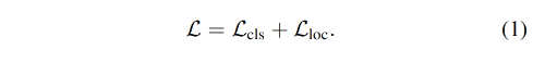
box classifier C C C 可以是简单的线性层,classification loss L c l s L_{cls} Lcls 可以被写为:

2、将目标检测重构为 phrase grounding:
不需要对每个 region/box 划分类别,grounding 任务是通过将每个 region 对齐(grounding/aligning) 到 text prompt 中的 c c c 个 phrase 上,如图 2 所示。
如何为 detection 任务设计 text prompt:将所有要检测的类别组成如下形式,每个类别名称都是需要被 grounded 的

在 grounding model 中,作者会计算 image region 和 words in prompt 之间的 alignment scores S g r o u n d S_{ground} Sground,
训练:将公式 2 中的 classification logits S c l s S_{cls} Scls 替换为 S g r o u n d S_{ground} Sground,然后最小化公式 1 和 2
注意,在公式 2 中, S g r o u n d ∈ R N × M S_{ground} \in R^{N \times M} Sground∈RN×M , T ∈ { 0 , 1 } N × c T\in\{0, 1\}^{N \times c} T∈{0,1}N×c,但由于 word token 的数量 M M M 一般都大于 phrases c c c 的数量,原因有四个:
所以,当 loss 是 binary sigmoid loss 时,将 T ∈ { 0 , 1 } N × c T\in\{0, 1\}^{N \times c} T∈{0,1}N×c 扩展为 T ′ ∈ { 0 , 1 } N × M T' \in\{0, 1\}^{N \times M} T′∈{0,1}N×M,这样就可以实现:
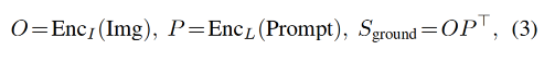
在公式 3 中,image 和 text 分别使用不同的 encoder 来提取特征,然后在最后进行融合来计算 alignment scores,这样的模型是 late-fusion models
在 vision-language 的相关方法中,deep fusion 很重要,能够优化 phrase grounding 模型
所以本文也使用了 deep fusion 的方式来对 image 和 language encoder 的结果进行融合,也就是在后面几个 encoder layer 就对 image 和 text 特征进行融合,如图 2 中间所示
作者使用 DyHead[10] 作为 image encoder,使用 BERT 作为 text encoder,则 deep-fused encoder 为:
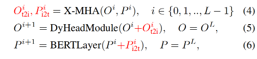
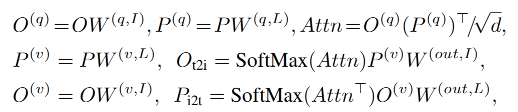
X-MHA 的每个 head 都计算从一个模态到另一个模态的 context vectors:
人工标注很费时费力,很多方法研究使用 self-training 方式来扩充,一般使用 teacher 模型来生成伪边界框来训练 student model,但生成的 label 也会受限于 concept pool,student model 也只能学习预设好的 concept pool。
本文的模型可以在 detection 和 grounding data 上同时训练,grounding data 可以提供丰富的语义信息来促进定位:
为什么 student model 的效果可能会超过 teacher model 的效果:
输入 prompt 长度的限制:
BERT 的长度限制是 512 token,在这里为了降低计算资源的消耗,将最大长度限制到了 256
当类别数量大于 token 限制时,作者会在训练和测试的时候都将类别拆分为多个 prompt,且证明了使用多 prompt 的方式只会带来很小的性能下降
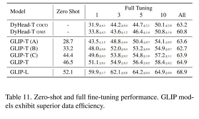
如图 2 所示,DyHead-T 在 Object365 上预训练,在 coco 上 zero-shot 的效果为 43.6,GLIP-T(A) 是以 grounding 格式实现的 DyHead,效果为 42.9。没有很大差别
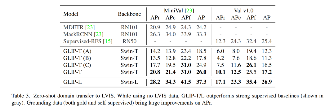
在测评 LVIS 时,LVIS 有 1000 个类别,作者在每个 prompt 中放 40 个类别,每次使用不同的 prompt 来测评对应的类别效果,
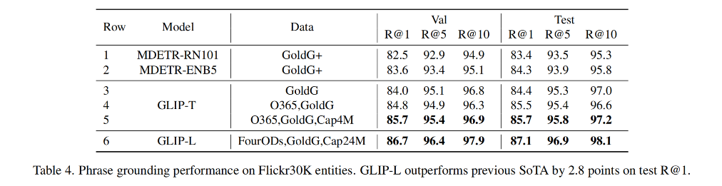
经过预训练的 GLIP 能够很方便的用于 grounding 和 detection 任务,作者在三个数据集上进行了验证:
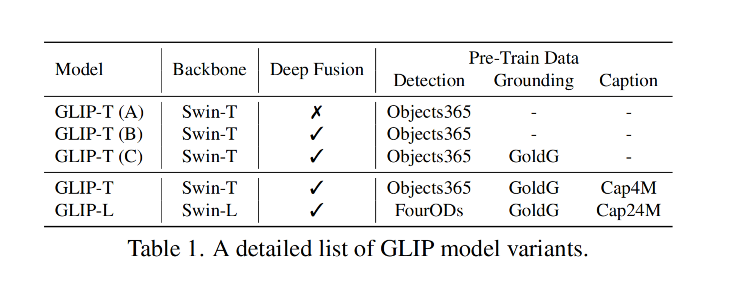
训练了 5 个 GLIP 变体,如表 1 所示:
DyHead:用于对比,先在 Object365 上训练 DyHead(因为 COCO 80 类基本包含在 Object 365),在推理的时候只推理 COCO 的 80 个类别
如表 2 所示:
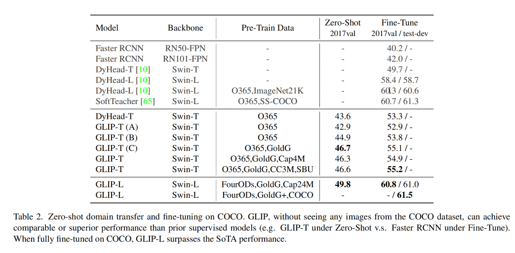
在 zero-shot 性能验证时,发现了 3 点:
GLIP 在所有类别上都表现出了很好的效果
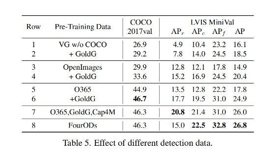
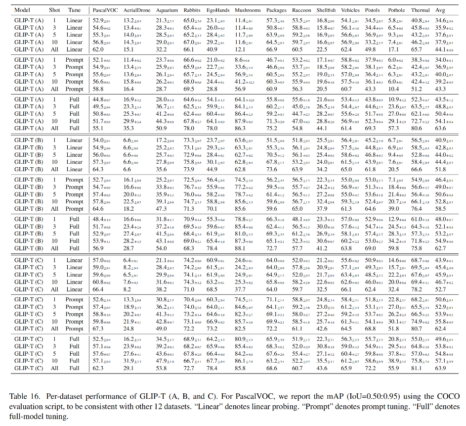
下表展示了在不同数据上预训练 GLIP-T 的消融实验:

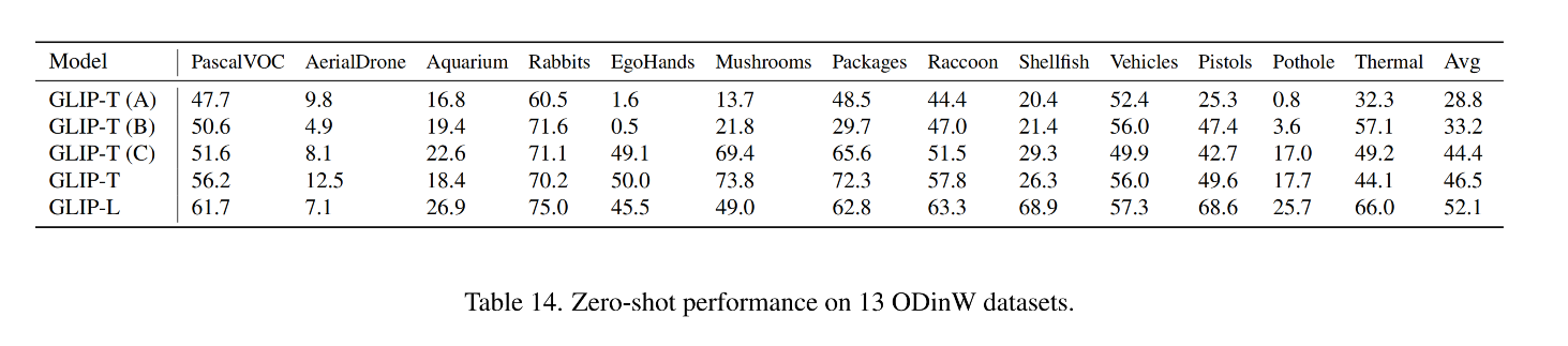
为了验证 GLIP 在 real-world 任务中的迁移能力,作者收集了一个 Object Detection in the wild(ODinW)集合,使用 13 个 Roboflow 上的 开源数据集。每个数据集关注的点不一样。EgoHands 需要定位人的手,Phthole 用于检测道路上的坑。
GLIP 能否迁移到不同域的任务呢:
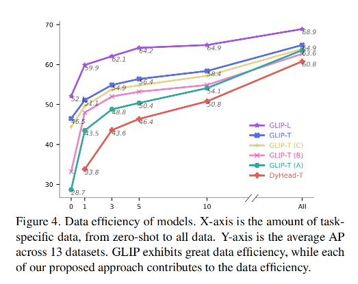
1、从数据来看
X-shot 就表示每个类别有 X 个训练样本
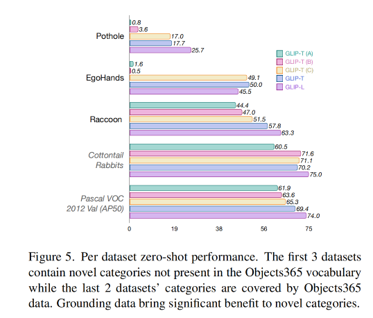
zero-shot 效果对比如下,引入 grounding data 能够提升对新概念类别的效果(如 Pothole 和 EgoHands),没有 grounding data 的模型(A 和 B)表现就较差,有 grounding data 的模型 C 表现就更好。
2、从微调来看,如何将一个模型扩展到所有任务
由于现在基础模型越来越大,如何降低部署的消耗就很重要
现在很多 language model、image classification、object detection 任务都是使用一个预训练好的模型,只修改少量需要定制的超参数就可以扩展到不同的任务上
如 linear probing[26]、prompt tuning[27]、efficient task adapter[13]
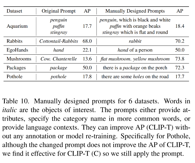
1、Manual prompt tuning
GLIP 支持在 prompt 中添加特定的 input 来指定不同的任务
如图 6,左侧表示模型无法识别 stingray,但如果添加上了一些属性 prompt(如 flat and round),模型就可以定位出 stingrays,AP50 从 4.6 提到了 9.7

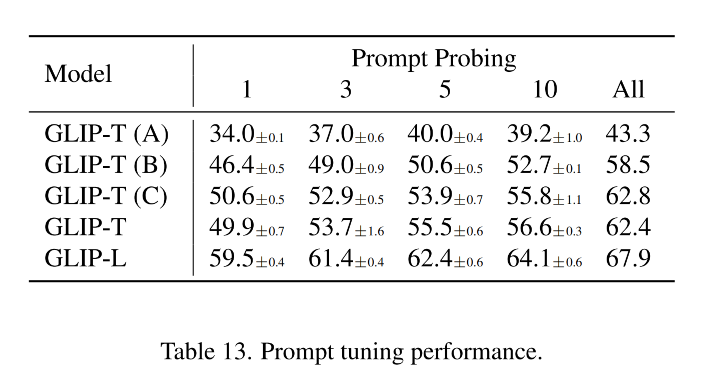
2、prompt tuning
GLIP 中,对目标检测任务,只 fine-tuning 两个部件:
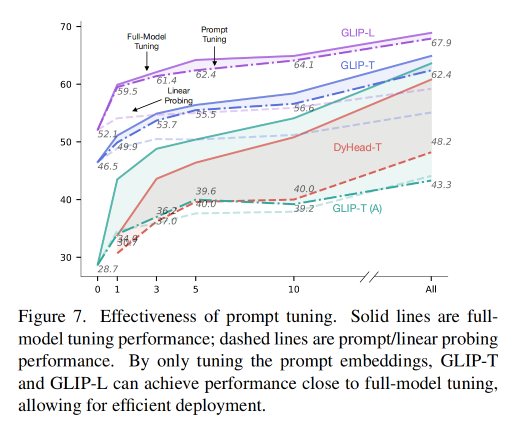
因为 language-aware 深层融合,GLIP 支持更有效且高效的迁移策略:prompt tuning
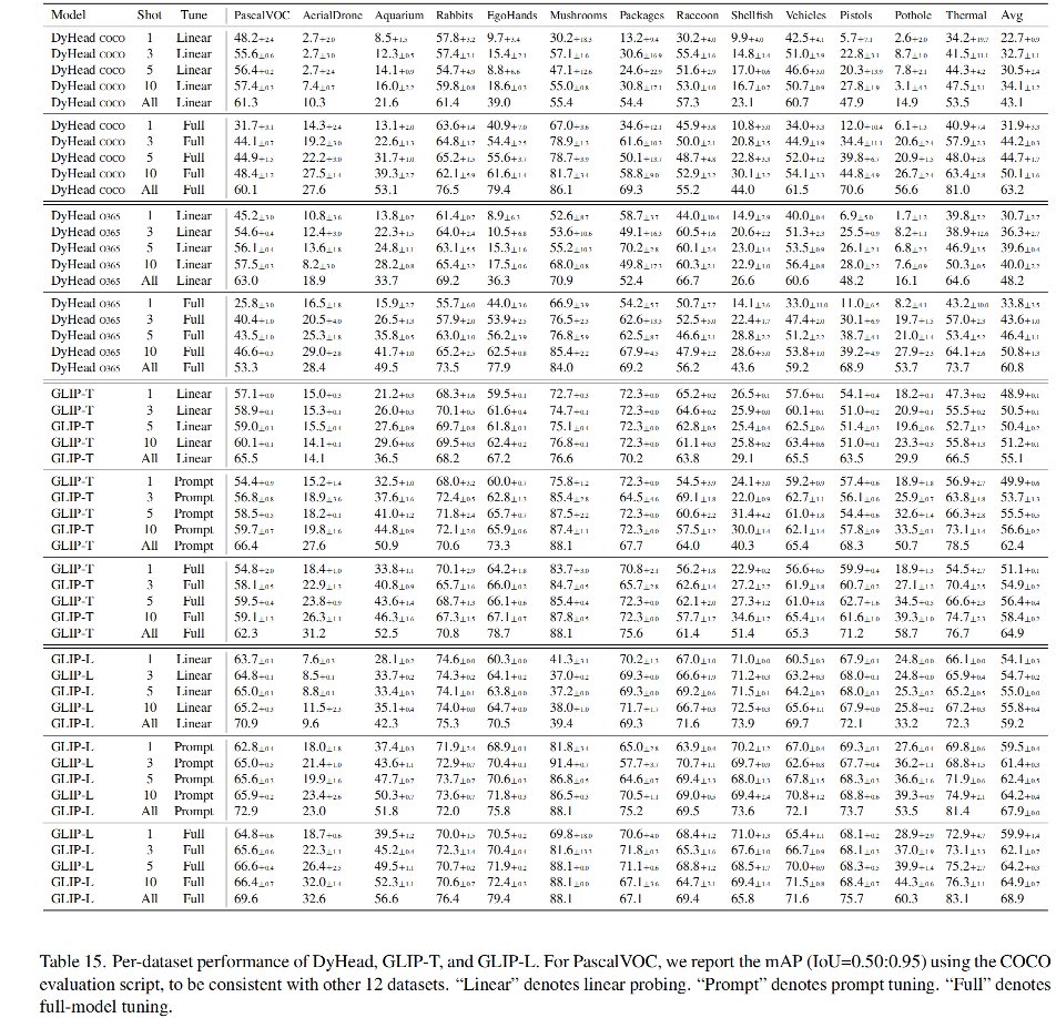
linear probing、prompt tuning、full-model tuning 这三种设置得到的结果如图 7 所示
拉取 docker 镜像,起 docker 来执行代码
# 拉取 docker 镜像
docker pull pengchuanzhang/pytorch:ubuntu20.04_torch1.9-cuda11.3-nccl2.9.9
# 起容器
sudo docker run --runtime=nvidia -it -d --name "xxx" -w /home/ -v /home:/home -e NVIDIA_VISIBLE_DEVICES=all --shm-size 128g pengchuanzhang/pytorch:ubuntu20.04_torch1.9-cuda11.3-nccl2.9.9 bash
# 安装环境
pip install einops shapely timm yacs tensorboardX ftfy prettytable pymongo -i http://pypi.douban.com/simple/ --trusted-host pypi.douban.com
pip install transformers -i http://pypi.douban.com/simple/ --trusted-host pypi.douban.com
python setup.py build develop --user
1、glip 预训练模型
https://huggingface.co/harold/GLIP/tree/main
2、语言预训练模型 bert
因为 glip 为多模态模型,所以需要前置语言模型,在代码中使用的是 transformer 库从 huggingface 中下载模型,但通常下不下来,可以在 huggingface 官网手动下载,然后将模型放入指定路径即可。
我这里找到了一个阿里源,下载的很快
① 在 glip 文件夹下新建一个 pretrained model 文件夹,然后使用如下命令,拉取对应的模型和 config
mkdir bert-base-uncased
wget -P bert-base-uncased https://thunlp.oss-cn-qingdao.aliyuncs.com/opennre/pretrain/bert-base-uncased/config.json
wget -P bert-base-uncased https://thunlp.oss-cn-qingdao.aliyuncs.com/opennre/pretrain/bert-base-uncased/pytorch_model.bin
wget -P bert-base-uncased https://thunlp.oss-cn-qingdao.aliyuncs.com/opennre/pretrain/bert-base-uncased/vocab.txt
② 在 glip/maskrcnn_benchmark/modeling/language_backbone/bert_model.py 中进行如下修改,被注释掉的是原本的代码,重写路径的是可执行的代码。
注意:有些博客中写可以在 from_pretraind 中指定 mirror 为清华源(mirror='https://mirrors.tuna.tsinghua.edu.cn/hugging-face-models'),这在 2021 年之后已经不可行了,所以最保险的方法就是自己手动下载模型,然后修改路径即可。
class BertEncoder(nn.Module):
    def __init__(self, cfg):
        super(BertEncoder, self).__init__()
        self.cfg = cfg
        self.bert_name = cfg.MODEL.LANGUAGE_BACKBONE.MODEL_TYPE
        print("LANGUAGE BACKBONE USE GRADIENT CHECKPOINTING: ", self.cfg.MODEL.LANGUAGE_BACKBONE.USE_CHECKPOINT)

        # if self.bert_name == "bert-base-uncased":
        #     config = BertConfig.from_pretrained(self.bert_name)
        #     config.gradient_checkpointing = self.cfg.MODEL.LANGUAGE_BACKBONE.USE_CHECKPOINT
        #     self.model = BertModel.from_pretrained(self.bert_name, add_pooling_layer=False, config=config)
        #     self.language_dim = 768
        if self.bert_name == "bert-base-uncased":
            config = BertConfig.from_pretrained('/glip/pretrained_models/bert-base-uncased')
            config.gradient_checkpointing = self.cfg.MODEL.LANGUAGE_BACKBONE.USE_CHECKPOINT
            self.model = BertModel.from_pretrained('/glip/pretrained_models/bert-base-uncased', add_pooling_layer=False, config=config)
            self.language_dim = 768
        elif self.bert_name == "roberta-base":
            config = RobertaConfig.from_pretrained(self.bert_name)
            config.gradient_checkpointing = self.cfg.MODEL.LANGUAGE_BACKBONE.USE_CHECKPOINT
            self.model = RobertaModel.from_pretrained(self.bert_name, add_pooling_layer=False, config=config)
            self.language_dim = 768
        else:
            raise NotImplementedError

        self.num_layers = cfg.MODEL.LANGUAGE_BACKBONE.N_LAYERS
1、COCO Evaluation
第一步:首先按如下方式对 COCO 数据进行组织:https://github.com/microsoft/GLIP/blob/main/DATA.md

即在 DATASET 中按如下方式放置 coco 数据集:

第二步:写 coco 对应的 yaml,configs/coco/val.yaml
MODEL:
  ATSS:
    NUM_CLASSES: 80 # these fields are not used; just a placeholder
  FCOS:
    NUM_CLASSES: 80
  ROI_BOX_HEAD:
    NUM_CLASSES: 80
  DYHEAD:
    NUM_CLASSES: 80
DATASETS:
  REGISTER:
    coco_train:
      img_dir: "coco/train2017"
      ann_file: "coco/annotations/instance_train2017.json"
    coco_val:
      img_dir: "coco/val2017/"
      ann_file: "coco/annotations/instances_val2017.json"
  TRAIN: ("coco_train",)
  TEST: ("coco_val",)

INPUT:
  MIN_SIZE_TRAIN: 800
  MAX_SIZE_TRAIN: 1333
  MIN_SIZE_TEST: 800
  MAX_SIZE_TEST: 1333
DATALOADER:
  SIZE_DIVISIBILITY: 32
  ASPECT_RATIO_GROUPING: False
TEST:
  IMS_PER_BATCH: 8
使用如下命令来测评:
python tools/test_grounding_net.py \
--config-file configs/pretrain/glip_Swin_T_O365_GoldG.yaml \
--task_config configs/coco/val.yaml \
--weight MODEL/glip_tiny_model_o365_goldg_cc_sbu.pth \
	TEST.IMS_PER_BATCH 1 \
	MODEL.DYHEAD.SCORE_AGG "MEAN" \
	TEST.EVAL_TASK detection \
	MODEL.DYHEAD.FUSE_CONFIG.MLM_LOSS False \
	OUTPUT_DIR {output_dir}
得到如下测评结果:mAP=46.6 (GroundingDino 为 48.5)
 Average Precision  (AP) @[ IoU=0.50:0.95 | area=   all | maxDets=100 ] = 0.46638
 Average Precision  (AP) @[ IoU=0.50      | area=   all | maxDets=100 ] = 0.63107
 Average Precision  (AP) @[ IoU=0.75      | area=   all | maxDets=100 ] = 0.50778
 Average Precision  (AP) @[ IoU=0.50:0.95 | area= small | maxDets=100 ] = 0.33602
 Average Precision  (AP) @[ IoU=0.50:0.95 | area=medium | maxDets=100 ] = 0.50633
 Average Precision  (AP) @[ IoU=0.50:0.95 | area= large | maxDets=100 ] = 0.59646
 Average Recall     (AR) @[ IoU=0.50:0.95 | area=   all | maxDets=  1 ] = 0.37554
 Average Recall     (AR) @[ IoU=0.50:0.95 | area=   all | maxDets= 10 ] = 0.62210
 Average Recall     (AR) @[ IoU=0.50:0.95 | area=   all | maxDets=100 ] = 0.65833
 Average Recall     (AR) @[ IoU=0.50:0.95 | area= small | maxDets=100 ] = 0.49174
 Average Recall     (AR) @[ IoU=0.50:0.95 | area=medium | maxDets=100 ] = 0.71016
 Average Recall     (AR) @[ IoU=0.50:0.95 | area= large | maxDets=100 ] = 0.81746
2023-07-10 09:52:15,449 maskrcnn_benchmark.inference INFO: OrderedDict([('bbox', OrderedDict([('AP', 0.4663779092127794), ('AP50', 0.6310650844926528), ('AP75', 0.50778317378933), ('APs', 0.33601965830665764), ('APm', 0.5063337770432529), ('APl', 0.5964644305214388)]))])
推理/测评流程图如下,推理代码是 engine/inference.py(line382):
第一步:这是 detection 测评任务,先生成 all_queries 和 all_positive_map_label_to_token
all_queries: 由类别名称组成的,用于文本输入,后面会对 queries 进行分词,然后使用语言模型提取特征
['person. bicycle. car. motorcycle. airplane. bus. train. truck. boat. traffic light. fire hydrant. stop sign. parking meter. bench. bird. cat. dog. horse. sheep. cow. elephant. bear. zebra. giraffe. backpack. umbrella. handbag. tie. suitcase. frisbee. skis. snowboard. sports ball. kite. baseball bat. baseball glove. skateboard. surfboard. tennis racket. bottle. wine glass. cup. fork. knife. spoon. bowl. banana. apple. sandwich. orange. broccoli. carrot. hot dog. pizza. donut. cake. chair. couch. potted plant. bed. dining table. toilet. tv. laptop. mouse. remote. keyboard. cell phone. microwave. oven. toaster. sink. refrigerator. book. clock. vase. scissors. teddy bear. hair drier. toothbrush']
all_positive_map_label_to_token: 是每个类别对应的编码的序号,如 1: [1] 表示类别 person 对应 tokenized 的 input_ids 中的第 1 个位置的编码。前面几个词语对应的都是 1、3、5、7、9…,没有出现 2、4、6、8 等位置,因为这些位置其实就是 . 的编码位置,还有 一些类别对应了两个或多个编码位置,如 10: [19, 20],可以看出 10 类对应的是 traffic light,本来就是两个单词,所以会对应多个位置。
也是测试时候用的 positive_map
[defaultdict(<class 'list'>, {1: [1], 2: [3], 3: [5], 4: [7], 5: [9], 6: [11], 7: [13], 8: [15], 9: [17], 10: [19, 20], 11: [22, 23, 24], 12: [26, 27], 13: [29, 30], 14: [32], 15: [34], 16: [36], 17: [38], 18: [40], 19: [42], 20: [44], 21: [46], 22: [48], 23: [50], 24: [52, 53, 54], 25: [56], 26: [58], 27: [60, 61], 28: [63], 29: [65], 30: [67, 68, 69], 31: [71, 72], 32: [74, 75], 33: [77, 78], 34: [80], 35: [82, 83], 36: [85, 86], 37: [88, 89], 38: [91, 92], 39: [94, 95, 96], 40: [98], 41: [100, 101], 42: [103], 43: [105], 44: [107], 45: [109], 46: [111], 47: [113], 48: [115], 49: [117], 50: [119], 51: [121, 122, 123], 52: [125], 53: [127, 128], 54: [130], 55: [132, 133], 56: [135], 57: [137], 58: [139], 59: [141, 142, 143], 60: [145], 61: [147, 148], 62: [150], 63: [152], 64: [154], 65: [156], 66: [158], 67: [160], 68: [162, 163], 69: [165], 70: [167], 71: [169, 170], 72: [172], 73: [174], 74: [176], 75: [178], 76: [180], 77: [182], 78: [184, 185], 79: [187, 188, 189], 80: [191, 192]})]
第二步:进入 detector/generalized_vl_rcnn.py(175) 执行模型 forward
第三步:对得到的所有类别、bbox_reg、centerness、anchor 等信息进行 grounding to object detection 特征的转换:
第四步:分类阈值过滤,即先每层分别处理得到每层保留得分大于阈值0.05的前1000个框
给框的分类得分(即dot_product_logits处理后的得分)乘 centerness 得分,用于过滤距离中心点远的框
之后,保留得分大于 self.pre_nms_thresh(0.05)的 anchor,然后保留前 1000 个 anchor
然后,使用 dot_product_logits[16400,80]、box 回归特征([16400,4]、nms 参数(前1000个)、anchors(16400个)这些特征来进行最终结果的过滤和保留
保留 anchor 中的得分大于 0.05 的前 1000 个框在 anchor 中的索引和预测类别,最终保留的预测结果就是 1000 个框
第五步:对保留的框进行 decode
使用预测的框和 anchor 来decode,decode 后就得到的是对每个 anchor 的修正后的结果,也就是预测框啦,具体怎么 decode 的呢
每层都解码完了后,就会得到这样的 bbox_list:[(BoxList(num_boxes=1000, image_width=1201, image_height=800, mode=xyxy), BoxList(num_boxes=877, image_width=1201, image_height=800, mode=xyxy), BoxList(num_boxes=313, image_width=1201, image_height=800, mode=xyxy), BoxList(num_boxes=0, image_width=1201, image_height=800, mode=xyxy), BoxList(num_boxes=0, image_width=1201, image_height=800, mode=xyxy))]
然后将所有层的 bbox_list 进行 concat,得到这样的:[BoxList(num_boxes=2190, image_width=1201, image_height=800, mode=xyxy)]
第六步:对所有保留下来的框中进行 NMS 过滤筛选(不分层级)(inference.py line750),NMS 阈值为 0.6,先直接进行 NMS 过滤,得到 BoxList(num_boxes=334, image_width=1201, image_height=800, mode=xyxy),即保留了 334 个框,但受限于每张图中最多的检出框个数(100),会保留前 100 个预测框。
2、LVIS Evaluation
3、ODinW / Custom Dataset Evaluation
4、Flickr30K Evaluation
finetuned 流程图如下:
在开始介绍代码之前,先介绍几个关键的问题:
1、输入 [img, text, target]
img:图像
text:所有要检测的类别名称组成的,coco 为例,需要将 coco 的标注信息转换成 grounding 任务能用的信息,即标签要有一个转换的过程(object detection to grounding 的过程)。具体执行转换的代码是 modulated_coco.py/CocoGrounding()
在 yaml 文件中会指定 SEPARATION_TOKENS: ". ",即类别之间使用 . 来分割
这些过程就在 make_data_loader 的时候执行了,所以不注意看很难发现
具体过程在 data/build.py/make_data_loader 中,所有超参数如下:
{'few_shot': 3, 'shuffle_seed': 3, 'random_sample_negative': 85, 'disable_shuffle': True, 'control_probabilities': (0.0, 0.0, 0.5, 0.0), 'separation_tokens': '. ', 'caption_min_box': 1, 'caption_conf': 0.9, 'caption_nms': 0.9, 'safeguard_positive_caption': True, 'local_debug': False, 'no_mask_for_od': False, 'no_mask_for_gold': False, 'mlm_obj_for_only_positive': False, 'caption_format_version': 'v1', 'special_safeguard_for_coco_grounding': False, 'diver_box_for_vqa': False, 'caption_prompt': None, 'use_caption_prompt': True, 'tokenizer': BertTokenizerFast(name_or_path='bert-base-uncased', vocab_size=30522, model_max_length=512, is_fast=True, padding_side='right', truncation_side='right', special_tokens={'unk_token': '[UNK]', 'sep_token': '[SEP]', 'pad_token': '[PAD]', 'cls_token': '[CLS]', 'mask_token': '[MASK]'}, clean_up_tokenization_spaces=True)}
data: {'factory': 'CocoGrounding', 'args': {'img_folder': './DATASET/coco/train2017', 'ann_file': './DATASET/coco/annotations/instances_train2017.json'}}
具体的负责操作的代码在 build.py(line93),也就是会进入 maskrcnn_benchmark.data.datasets.modulated_coco.CocoGrounding
处理后的标签如下,也就是将 OD 的标签转换成了 grounding 任务能用的标签了:
'person. bicycle. car. motorcycle. airplane. bus. train. truck. boat. traffic light. fire hydrant. stop sign. parking meter. bench. bird. cat. dog. horse. sheep. cow. elephant. bear. zebra. giraffe. backpack. umbrella. handbag. tie. suitcase. frisbee. skis. snowboard. sports ball. kite. baseball bat. baseball glove. skateboard. surfboard. tennis racket. bottle. wine glass. cup. fork. knife. spoon. bowl. banana. apple. sandwich. orange. broccoli. carrot. hot dog. pizza. donut. cake. chair. couch. potted plant. bed. dining table. toilet. tv. laptop. mouse. remote. keyboard. cell phone. microwave. oven. toaster. sink. refrigerator. book. clock. vase. scissors. teddy bear. hair drier. toothbrush'
target:标签,包括图像中的目标框的位置、类别
2、text 需要怎么处理成目标检测可用的 label 的
self.tokenizer.batch_encode_plus 对其进行序列化(分词),会输出以下三个部分,序列化后的特征会用于后续编码,如将某个框的类别编码成 256 维的特征,对应的就是 input_ids 中的类别编号
input_ids:101 是 [CLS],102 是 [SEP],分别表示头和尾
2711、1012、10165 是 bert-base-uncased有个json文件,里面是所有字符。7592这种应该是该字符所在的行数(从 0 开始计算行数)
如 2712 对应 person,1012对应 . ,11868 是 tooth,18623 是 ##brush,即会把组成的词语拆开成两个甚至多个,
input_ids 就表示了对 caption 的所有类别进行了编码,编码成文本 txt 中的行号,具体的可以查看 json 文件。然后将编码后的特征输入 language_backbone 进行特征提取。
input_ids 的维度为 [4, 256],也就是将每个图像的 caption 都进行编码,包括caption 中的单词和 . ,这里有 194 个非零值,因为组合单词会占多个位置,留下了 62 个 0 的位置,就是没用到的 token 位置。
input_ids: [ 101, 2711, 1012, 10165, 1012, 2482, 1012, 9055, 1012, 13297, 1012, 3902, 1012, 3345, 1012, 4744, 1012, 4049, 1012, 4026, 2422, 1012, 2543, 26018, 3372, 1012, 2644, 3696, 1012, 5581, 8316, 1012, 6847, 1012, 4743, 1012, 4937, 1012, 3899, 1012, 3586, 1012, 8351, 1012, 11190, 1012, 10777, 1012, 4562, 1012, 29145, 1012, 21025, 27528, 7959, 1012, 13383, 1012, 12977, 1012, 2192, 16078, 1012, 5495, 1012, 15940, 1012, 10424, 2483, 11306, 1012, 8301, 2015, 1012, 4586, 6277, 1012, 2998, 3608, 1012, 20497, 1012, 3598, 7151, 1012, 3598, 15913, 1012, 17260, 6277, 1012, 14175, 6277, 1012, 5093, 14513, 3388, 1012, 5835, 1012, 4511, 3221, 1012, 2452, 1012, 9292, 1012, 5442, 1012, 15642, 1012, 4605, 1012, 15212, 1012, 6207, 1012, 11642, 1012, 4589, 1012, 22953, 21408, 3669, 1012, 25659, 1012, 2980, 3899, 1012, 10733, 1012, 2123, 4904, 1012, 9850, 1012, 3242, 1012, 6411, 1012, 8962, 3064, 3269, 1012, 2793, 1012, 7759, 2795, 1012, 11848, 1012, 2694, 1012, 12191, 1012, 8000, 1012, 6556, 1012, 9019, 1012, 3526, 3042, 1012, 18302, 1012, 17428, 1012, 15174, 2121, 1012, 7752, 1012, 18097, 1012, 2338, 1012, 5119, 1012, 18781, 1012, 25806, 1012, 11389, 4562, 1012, 2606, 2852, 3771, 1012, 11868, 18623, 102, 0, 0, 0, 0, 0, 0, 0, 0, 0, 0, 0, 0, 0, 0, 0, 0, 0, 0, 0, 0, 0, 0, 0, 0, 0, 0, 0, 0, 0, 0, 0, 0, 0, 0, 0, 0, 0, 0, 0, 0, 0, 0, 0, 0, 0, 0, 0, 0, 0, 0, 0, 0, 0, 0, 0, 0, 0, 0, 0, 0, 0, 0]
token_type_ids:表示单词属于哪个句子,第一个句子为 0,第二句子为1。
[0, 0, 0, 0, 0, 0, 0, 0, 0, 0, 0, 0, 0, 0, 0, 0, 0, 0, 0, 0, 0, 0, 0, 0, 0, 0, 0, 0, 0, 0, 0, 0, 0, 0, 0, 0, 0, 0, 0, 0, 0, 0, 0, 0, 0, 0, 0, 0, 0, 0, 0, 0, 0, 0, 0, 0, 0, 0, 0, 0, 0, 0, 0, 0, 0, 0, 0, 0, 0, 0, 0, 0, 0, 0, 0, 0, 0, 0, 0, 0, 0, 0, 0, 0, 0, 0, 0, 0, 0, 0, 0, 0, 0, 0, 0, 0, 0, 0, 0, 0, 0, 0, 0, 0, 0, 0, 0, 0, 0, 0, 0, 0, 0, 0, 0, 0, 0, 0, 0, 0, 0, 0, 0, 0, 0, 0, 0, 0, 0, 0, 0, 0, 0, 0, 0, 0, 0, 0, 0, 0, 0, 0, 0, 0, 0, 0, 0, 0, 0, 0, 0, 0, 0, 0, 0, 0, 0, 0, 0, 0, 0, 0, 0, 0, 0, 0, 0, 0, 0, 0, 0, 0, 0, 0, 0, 0, 0, 0, 0, 0, 0, 0, 0, 0, 0, 0, 0, 0, 0, 0, 0, 0, 0, 0]
attention_mask:维度也是 256 维的,1 表示有 phrase,0 表示空位
[1, 1, 1, 1, 1, 1, 1, 1, 1, 1, 1, 1, 1, 1, 1, 1, 1, 1, 1, 1, 1, 1, 1, 1, 1, 1, 1, 1, 1, 1, 1, 1, 1, 1, 1, 1, 1, 1, 1, 1, 1, 1, 1, 1, 1, 1, 1, 1, 1, 1, 1, 1, 1, 1, 1, 1, 1, 1, 1, 1, 1, 1, 1, 1, 1, 1, 1, 1, 1, 1, 1, 1, 1, 1, 1, 1, 1, 1, 1, 1, 1, 1, 1, 1, 1, 1, 1, 1, 1, 1, 1, 1, 1, 1, 1, 1, 1, 1, 1, 1, 1, 1, 1, 1, 1, 1, 1, 1, 1, 1, 1, 1, 1, 1, 1, 1, 1, 1, 1, 1, 1, 1, 1, 1, 1, 1, 1, 1, 1, 1, 1, 1, 1, 1, 1, 1, 1, 1, 1, 1, 1, 1, 1, 1, 1, 1, 1, 1, 1, 1, 1, 1, 1, 1, 1, 1, 1, 1, 1, 1, 1, 1, 1, 1, 1, 1, 1, 1, 1, 1, 1, 1, 1, 1, 1, 1, 1, 1, 1, 1, 1, 1, 1, 1, 1, 1, 1, 1, 1, 1, 1, 1, 1, 1, 0, 0, 0, 0, 0, 0, 0, 0, 0, 0, 0, 0, 0, 0, 0, 0, 0, 0, 0, 0, 0, 0, 0, 0, 0, 0, 0, 0, 0, 0, 0, 0, 0, 0, 0, 0, 0, 0, 0, 0, 0, 0, 0, 0, 0, 0, 0, 0, 0, 0, 0, 0, 0, 0, 0, 0, 0, 0, 0, 0, 0, 0]
3、分词后的特征怎么提取文本特征
4、targets 长什么样子
[BoxList(num_boxes=4, image_width=640, image_height=968, mode=xyxy), BoxList(num_boxes=4, image_width=800, image_height=1210, mode=xyxy), BoxList(num_boxes=2, image_width=800, image_height=1064, mode=xyxy), BoxList(num_boxes=2, image_width=800, image_height=1199, mode=xyxy)]tatgets[0].bbox:tensor([[310.1792, 241.7580, 427.6033, 419.7641], [236.5868, 86.9536, 353.6931, 421.2010], [418.5555, 123.3293, 543.2572, 398.0749], [ 77.2827, 117.1431, 543.6808, 912.5518]], device='cuda:0')
targets[0].get_field('labels'):tensor([80, 80, 80, 42], device='cuda:0')
4、很重要的 positive_map 又是什么
纵观整个代码,出现频率很高的还有 positive_map ,创建的位置:data/datasets/modulated_coco.py(line561)
positive_map 长什么样子:[0,0,0,...,1,0],...,[0,1,0,...,0]
positive_map 是什么:我们前面知道了 target 中包含每个框的类别信息,还知道了 BERT 会将每个输入 phrase 编码为 256 维的特征向量,那么每个框的类别信息也就可以用一个 256 维的特征向量来表示,而不是像传统目标检测方法中直接使用一个 ‘person’ 的字符串来表示啦。
所以 positive_map 就是一个大小为 [目标个数,256] 的特征,每一行都表示该目标的类别,而这里的类别编码也会映射回前面 tokenized 后的 input_ids,即类别编码和类别编号是一一对应的。
positive_map 会作用于 anchor,即 anchor 经过 ATSS 分配后就有了类别信息(源于其对应的 gt),那么将 positive_map 和 anchor 进行组合,就能将 anchor 的类别映射到 256 维的编码。
positive_map 的作用:给 anchor 分配类别编码,然后作为真值参与 loss 的计算:
1、COCO Fine-tuning
python -m torch.distributed.launch --nproc_per_node=4 --master_port=10801 tools/finetune.py \
      --config-file configs/pretrain/glip_Swin_T_O365_GoldG.yaml --skip-test \
      --custom_shot_and_epoch_and_general_copy 3_200_4 \
      --evaluate_only_best_on_test --push_both_val_and_test \
      DATASETS.TRAIN '("coco_grounding_train", )' \
      MODEL.WEIGHT MODEL/glip_tiny_model_o365_goldg_cc_sbu.pth \
      SOLVER.USE_AMP True TEST.DURING_TRAINING True TEST.IMS_PER_BATCH 4 SOLVER.IMS_PER_BATCH 4 SOLVER.WEIGHT_DECAY 0.05 TEST.EVAL_TASK detection MODEL.BACKBONE.FREEZE_CONV_BODY_AT 2 MODEL.DYHEAD.USE_CHECKPOINT True SOLVER.FIND_UNUSED_PARAMETERS False SOLVER.TEST_WITH_INFERENCE True SOLVER.USE_AUTOSTEP True DATASETS.USE_OVERRIDE_CATEGORY True SOLVER.SEED 10 DATASETS.SHUFFLE_SEED 3 DATASETS.USE_CAPTION_PROMPT True DATASETS.DISABLE_SHUFFLE True \
      SOLVER.STEP_PATIENCE 3 SOLVER.CHECKPOINT_PER_EPOCH 1.0 SOLVER.AUTO_TERMINATE_PATIENCE 8 SOLVER.MODEL_EMA 0.0 SOLVER.TUNING_HIGHLEVEL_OVERRIDE full
custom_shot_and_epoch_and_general_copy 是指定不同的 shot tuning、epoch、general copy 的
2、COCO promot tuning
python -m torch.distributed.launch --nproc_per_node=4 --master_port=10831 tools/finetune.py \
      --config-file configs/pretrain/glip_Swin_T_O365_GoldG.yaml --skip-test \
      --custom_shot_and_epoch_and_general_copy 3_200_4 \
      --evaluate_only_best_on_test --push_both_val_and_test \
      DATASETS.TRAIN '("coco_grounding_train", )' \
      MODEL.WEIGHT MODEL/glip_tiny_model_o365_goldg_cc_sbu.pth \
      SOLVER.USE_AMP True TEST.DURING_TRAINING True TEST.IMS_PER_BATCH 4 SOLVER.IMS_PER_BATCH 4 SOLVER.BASE_LR 0.05 SOLVER.WEIGHT_DECAY 0.25 TEST.EVAL_TASK detection MODEL.BACKBONE.FREEZE_CONV_BODY_AT 2 MODEL.DYHEAD.USE_CHECKPOINT True SOLVER.FIND_UNUSED_PARAMETERS False SOLVER.TEST_WITH_INFERENCE True SOLVER.USE_AUTOSTEP True DATASETS.USE_OVERRIDE_CATEGORY True SOLVER.SEED 10 DATASETS.SHUFFLE_SEED 3 DATASETS.USE_CAPTION_PROMPT True DATASETS.DISABLE_SHUFFLE True \
      SOLVER.STEP_PATIENCE 3 SOLVER.CHECKPOINT_PER_EPOCH 1.0 SOLVER.AUTO_TERMINATE_PATIENCE 8 SOLVER.MODEL_EMA 0.0 SOLVER.TUNING_HIGHLEVEL_OVERRIDE language_prompt_v2
和 fine-tuning 的主要区别在于:
SOLVER.BASE_LR 0.05SOLVER.WEIGHT_DECAY 0.25SOLVER.TUNING_HIGHLEVEL_OVERRIDE language_prompt_v2可以去代码里边看一下 SOLVER.TUNING_HIGHLEVEL_OVERRIDE 的设计:tools/finetune.py(line215)
def tuning_highlevel_override(cfg,):
    if cfg.SOLVER.TUNING_HIGHLEVEL_OVERRIDE == "full":
        cfg.MODEL.BACKBONE.FREEZE = False
        cfg.MODEL.FPN.FREEZE = False
        cfg.MODEL.RPN.FREEZE = False
        cfg.MODEL.LINEAR_PROB = False
        cfg.MODEL.DYHEAD.FUSE_CONFIG.ADD_LINEAR_LAYER = False
        cfg.MODEL.LANGUAGE_BACKBONE.FREEZE = False
    elif cfg.SOLVER.TUNING_HIGHLEVEL_OVERRIDE == "linear_prob":
        cfg.MODEL.BACKBONE.FREEZE = True
        cfg.MODEL.FPN.FREEZE = True
        cfg.MODEL.RPN.FREEZE = False
        cfg.MODEL.LINEAR_PROB = True
        cfg.MODEL.DYHEAD.FUSE_CONFIG.ADD_LINEAR_LAYER = False
        cfg.MODEL.LANGUAGE_BACKBONE.FREEZE = True
        cfg.MODEL.LANGUAGE_BACKBONE.FREEZE = True
        cfg.MODEL.DYHEAD.USE_CHECKPOINT = False # Disable checkpoint
    elif cfg.SOLVER.TUNING_HIGHLEVEL_OVERRIDE == "language_prompt_v1":
        cfg.MODEL.BACKBONE.FREEZE = True
        cfg.MODEL.FPN.FREEZE = True
        cfg.MODEL.RPN.FREEZE = True
        cfg.MODEL.LINEAR_PROB = False
        cfg.MODEL.DYHEAD.FUSE_CONFIG.ADD_LINEAR_LAYER = False
        cfg.MODEL.LANGUAGE_BACKBONE.FREEZE = False
    elif cfg.SOLVER.TUNING_HIGHLEVEL_OVERRIDE == "language_prompt_v2":
        cfg.MODEL.BACKBONE.FREEZE = True
        cfg.MODEL.FPN.FREEZE = True
        cfg.MODEL.RPN.FREEZE = True
        cfg.MODEL.LINEAR_PROB = False
        cfg.MODEL.DYHEAD.FUSE_CONFIG.ADD_LINEAR_LAYER = True
        cfg.MODEL.LANGUAGE_BACKBONE.FREEZE = True
    elif cfg.SOLVER.TUNING_HIGHLEVEL_OVERRIDE == "language_prompt_v3":
        cfg.MODEL.BACKBONE.FREEZE = True
        cfg.MODEL.FPN.FREEZE = True
        cfg.MODEL.RPN.FREEZE = True
        cfg.MODEL.LINEAR_PROB = True # Turn on linear probe
        cfg.MODEL.DYHEAD.FUSE_CONFIG.ADD_LINEAR_LAYER = False
        cfg.MODEL.LANGUAGE_BACKBONE.FREEZE = False # Turn on language backbone
    elif cfg.SOLVER.TUNING_HIGHLEVEL_OVERRIDE == "language_prompt_v4":
        cfg.MODEL.BACKBONE.FREEZE = True
        cfg.MODEL.FPN.FREEZE = True
        cfg.MODEL.RPN.FREEZE = True
        cfg.MODEL.LINEAR_PROB = True # Turn on linear probe
        cfg.MODEL.DYHEAD.FUSE_CONFIG.ADD_LINEAR_LAYER = True
        cfg.MODEL.LANGUAGE_BACKBONE.FREEZE = True # Turn off language backbone
    return cfg
3、ODinW / Custom Dataset Fine-Tuning
训练代码位置:finetune.py→maskrcnn_benchmark/engine/trainer.py(line45) → maskrcnn_benchmark/modeling/generalized_vl_rcnn.py(line134),这里对 model 中需要冻结的层进行冻结
冻结完成后进行本次迭代所需的 images 和 label 等的提取,maskrcnn_benchmark/engine/trainer.py(line45)
maskrcnn_benchmark/modeling/detector/generalized_vl_rcnn.py(175) 训练 forward
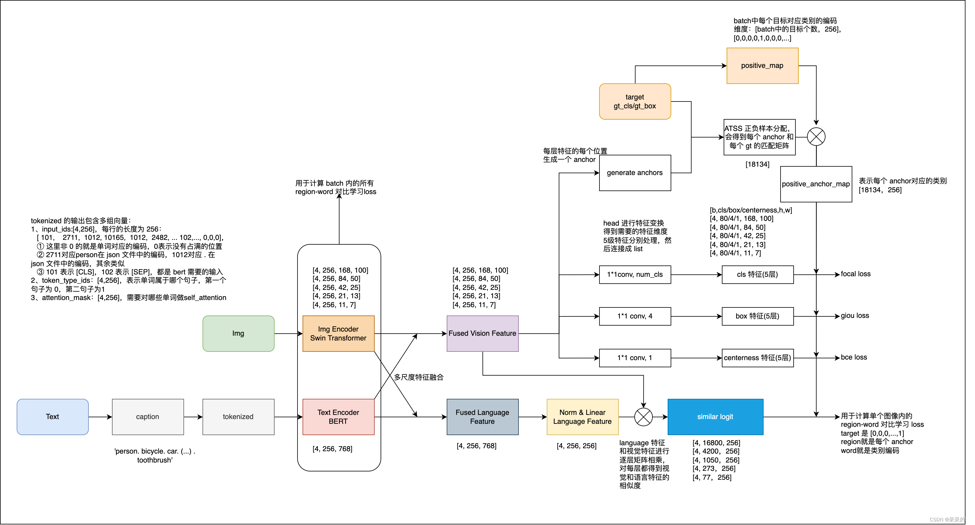
先对 language 编码进行 tokenized,使用函数为 batch_encode_plus,输出包括
input_ids:[4, 256],是单词在词典中的编码,4 是 batch,256 是文本 token 的最大长度token_type_ids:[4, 256],区分两个句子的编码(上句全为0,下句全为1)attention_mask:[4, 256],指定对哪些词进行self-Attention操作special_token_mask:[4, 256]caption:'person. bicycle. car. motorcycle. airplane. bus. train. truck. boat. traffic light. fire hydrant. stop sign. parking meter. bench. bird. cat. dog. horse. sheep. cow. elephant. bear. zebra. giraffe. backpack. umbrella. handbag. tie. suitcase. frisbee. skis. snowboard. sports ball. kite. baseball bat. baseball glove. skateboard. surfboard. tennis racket. bottle. wine glass. cup. fork. knife. spoon. bowl. banana. apple. sandwich. orange. broccoli. carrot. hot dog. pizza. donut. cake. chair. couch. potted plant. bed. dining table. toilet. tv. laptop. mouse. remote. keyboard. cell phone. microwave. oven. toaster. sink. refrigerator. book. clock. vase. scissors. teddy bear. hair drier. toothbrush'
language 编码完后得到 language_dict_features
language_dict_features['aggregate']:[4, 768]language_dict_features['embedded']:[4, 256, 768],256 是 token 长度,768 是 bert 会将每个 单词转换为 768 维的向量language_dict_features['masks']:[4, 256]language_dict_features['hidden']:[4, 256, 768]然后对 visual 特征使用 visual backbone 进行提取(swin),得到 5 层不同层级的 swin 特征,尺度分别为:[4, 256, 92, 136], [4, 256, 46, 68],[4, 256, 23, 34],[4, 256, 12, 17],[4, 256, 6, 9]
之后再使用 attention,对图像特征、语言特征进行融合maskrcnn_benchmark/modeling/rpn/vldyhead.py(892)→line(560)
使用 early fusion module 对两组特征进行 fuse(MHS-A/MHS-B),visual 特征是 5 级,language 特征是 5 种,特征融合是代码如下,是对图像的 5 级特征和 language 的 hidden/mask 特征进行融合,这里的多级融合也就是的不同层级的 swin transformer 特征和 language 特征进行融合,而不是只使用某一级进行融合。融合之后得到的特征和融合之前的特征大小是一样的,视觉特征为 [4, 256, 92, 136], [4, 256, 46, 68],[4, 256, 23, 34],[4, 256, 12, 17],[4, 256, 6, 9],语言特征为 [4, 256, 768],融合后的语言特征更新到 language_dict_features['hidden'] 中。
对语言特征进行规范化和一些线性操作
对视觉特征来提取分类、回归、centerness 特征、对每个层级的特征和语言特征进行相似性度量
生成 anchor,[[BoxList(num_boxes=16800, image_width=720, image_height=1283, mode=xyxy), BoxList(num_boxes=4200, image_width=720, image_height=1283, mode=xyxy), BoxList(num_boxes=1050, image_width=720, image_height=1283, mode=xyxy), BoxList(num_boxes=273, image_width=720, image_height=1283, mode=xyxy), BoxList(num_boxes=77, image_width=720, image_height=1283, mode=xyxy)], [BoxList(num_boxes=16800, image_width=748, image_height=1333, mode=xyxy), BoxList(num_boxes=4200, image_width=748, image_height=1333, mode=xyxy), BoxList(num_boxes=1050, image_width=748, image_height=1333, mode=xyxy), BoxList(num_boxes=273, image_width=748, image_height=1333, mode=xyxy), BoxList(num_boxes=77, image_width=748, image_height=1333, mode=xyxy)], [BoxList(num_boxes=16800, image_width=560, image_height=839, mode=xyxy), BoxList(num_boxes=4200, image_width=560, image_height=839, mode=xyxy), BoxList(num_boxes=1050, image_width=560, image_height=839, mode=xyxy), BoxList(num_boxes=273, image_width=560, image_height=839, mode=xyxy), BoxList(num_boxes=77, image_width=560, image_height=839, mode=xyxy)], [BoxList(num_boxes=16800, image_width=800, image_height=1147, mode=xyxy), BoxList(num_boxes=4200, image_width=800, image_height=1147, mode=xyxy), BoxList(num_boxes=1050, image_width=800, image_height=1147, mode=xyxy), BoxList(num_boxes=273, image_width=800, image_height=1147, mode=xyxy), BoxList(num_boxes=77, image_width=800, image_height=1147, mode=xyxy)]]
对 batch 中的 label 进行信息提取(loss.py line653),以一张图为例,bboxes_per_im = targets_per_im.bbox,labels_per_im = targets_per_im.get_field("labels"), num_gt = len(bboxes_per_im)
tensor([[282.8400, 263.7800, 319.6100, 296.5700], [ 21.1700, 30.2600, 449.5800, 457.6000], [122.3300, 129.2700, 429.1300, 471.5900], [235.6900, 338.0400, 257.0000, 366.4200]], device='cuda:0')
tensor([80, 1, 1, 80], device='cuda:0')
对 anchor 和 labels 求 iou,每个 anchor 和每个 gt 都得到一个 iou
求 anchor 和 每个 gt 的中心点的距离(不区分层级,所有层级的anchor都和 gt 计算距离),然后以每个层级分别基于两者之间的距离来选择哪些 anchor 保留,每个 gt 保留和其距离最近的前 9 个 anchor(就是 ATSS 的分配方式),求得保留下来的 anchor 对应的 iou 的均值和方差,将 iou>均值+方差的 anchor 设置为正,其他设置为负 anchor,如果一个 anchor 被分配到多个 gt 上去了,则只将其分配到 iou 最大的 gt 上去,并且按 gt 类别给其对应的 anchor 分配类别
根据保留的 anchor 和对应的 box、cls、token、centerness,分别求对应的 loss
{'loss_reg': tensor(0.1464, device='cuda:0', grad_fn=<MulBackward0>), 'loss_centerness': tensor(0.6058, device='cuda:0', grad_fn=<DivBackward0>), 'loss_cls': tensor(0., device='cuda:0', grad_fn=<MulBackward0>)}
{' 'loss_dot_product_token': tensor(0.3043, device='cuda:0', grad_fn=<MulBackward0>)}
1、Download ODinW
2、(Zero-Shot) Evaluation
3、Full-Model Fine-Tuning
4、Prompt Tuning
5、Linear Probing
6、Knowledge-Augmented Inference
推理可视化过程如下:
{'input_ids': tensor([[ 101, 3960, 3468, 4641, 2006, 2327, 1997, 1996, 11142, 102]]), 'token_type_ids': tensor([[0, 0, 0, 0, 0, 0, 0, 0, 0, 0]]), 'attention_mask': tensor([[1, 1, 1, 1, 1, 1, 1, 1, 1, 1]])}
['bobble heads', 'top', 'the shelf'],这些分后的词就是要检测的 label,如果输入 caption 为 'sofa . remote . dog . person . car . sky . plane .',则 nltk 处理后就是 noun_phrases:['sofa', 'remote', 'dog', 'person', 'car', 'sky', 'plane']
[[[0, 12]], [[16, 19]], [[23, 32]]],然后将要得到 3x256 的 positive_map(这个 3 是因为前面提取了 3 个 phrase)。方法是,对于第一组 [0,12],对 0 和 12 分别进行 tokenized.char_to_token(0) 和 tokenized.char_to_token(12-1) ,得到 beg_pos 和 end_pos,将每个 phrase 编码到 256 维特征,然后找到 256 维特征中 1 的位置,得到 positive_map_label_to_token :{1: [1, 2, 3], 2: [5], 3: [7, 8]}
BoxList(num_boxes=13, image_width=640, image_height=480, mode=xyxy),再把预测结果 resize 到原图大小,predictions.get_field("labels").tolist(): [1, 1, 1, 3, 1, 2, 1, 3, 1, 1, 2, 3, 1],输出 scores:predictions.get_field("scores"):tensor([0.2432, 0.3272, 0.2529, 0.3403, 0.7509, 0.3260, 0.2384, 0.2128, 0.1887, 0.4218, 0.3763, 0.7082, 0.1189])如设置可视化阈值为 0.5,则保留得分大于 0.5 的框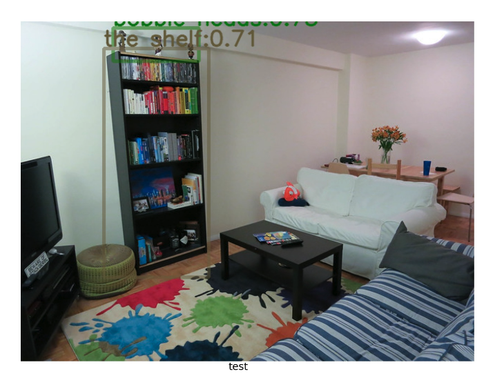
在得到图像的多级特征后,要给每个特征图的每个位置生成一个 anchor,那 anchor 是怎么生成的呢
[[-448., -448., 575., 575.], [-320., -448., 703., 575], [-192., -448., 831., 575.], [ -64., -448., 959., 575.], [ 64., -448., 1087., 575.], [ 192., -448., 1215., 575.], [ 320., -448., 1343., 575.],...],这里的数字其实是以原始图像坐标为标准的坐标# maskrcnn_benchmark/modeling/rpn/anchor_generator.py(113)forward()
def forward(self, image_list, feature_maps):
grid_sizes = [feature_map.shape[-2:] for feature_map in feature_maps]
# [torch.Size([92, 140]), torch.Size([46, 70]), torch.Size([23, 35]), torch.Size([12, 18]), torch.Size([6, 9])]
anchors_over_all_feature_maps = self.grid_anchors(grid_sizes)
anchors = []
if isinstance(image_list, ImageList):
for i, (image_height, image_width) in enumerate(image_list.image_sizes):
anchors_in_image = []
for anchors_per_feature_map in anchors_over_all_feature_maps:
boxlist = BoxList(
anchors_per_feature_map, (image_width, image_height), mode="xyxy"
)
self.add_visibility_to(boxlist)
anchors_in_image.append(boxlist)
anchors.append(anchors_in_image)
else:
image_height, image_width = [int(x) for x in image_list.size()[-2:]]
anchors_in_image = []
for anchors_per_feature_map in anchors_over_all_feature_maps:
boxlist = BoxList(
anchors_per_feature_map, (image_width, image_height), mode="xyxy"
)
self.add_visibility_to(boxlist)
anchors_in_image.append(boxlist)
anchors.append(anchors_in_image)
return anchors
VLDyHeadModule(
  (head): VLDyHead(
    (dyhead_tower): Sequential(
      (0): VLFuse(
        (b_attn): BiAttentionBlockForCheckpoint(
          (layer_norm_v): LayerNorm((256,), eps=1e-05, elementwise_affine=True)
          (layer_norm_l): LayerNorm((768,), eps=1e-05, elementwise_affine=True)
          (attn): BiMultiHeadAttention(
            (v_proj): Linear(in_features=256, out_features=2048, bias=True)
            (l_proj): Linear(in_features=768, out_features=2048, bias=True)
            (values_v_proj): Linear(in_features=256, out_features=2048, bias=True)
            (values_l_proj): Linear(in_features=768, out_features=2048, bias=True)
            (out_v_proj): Linear(in_features=2048, out_features=256, bias=True)
            (out_l_proj): Linear(in_features=2048, out_features=768, bias=True)
          )
          (drop_path): Identity()
        )
      )
      (1): BertEncoderLayer(
        (attention): BertAttention(
          (self): BertSelfAttention(
            (query): Linear(in_features=768, out_features=768, bias=True)
            (key): Linear(in_features=768, out_features=768, bias=True)
            (value): Linear(in_features=768, out_features=768, bias=True)
            (dropout): Dropout(p=0.1, inplace=False)
          )
          (output): BertSelfOutput(
            (dense): Linear(in_features=768, out_features=768, bias=True)
            (LayerNorm): LayerNorm((768,), eps=1e-12, elementwise_affine=True)
            (dropout): Dropout(p=0.1, inplace=False)
          )
        )
        (intermediate): BertIntermediate(
          (dense): Linear(in_features=768, out_features=3072, bias=True)
          (intermediate_act_fn): GELUActivation()
        )
        (output): BertOutput(
          (dense): Linear(in_features=3072, out_features=768, bias=True)
          (LayerNorm): LayerNorm((768,), eps=1e-12, elementwise_affine=True)
          (dropout): Dropout(p=0.1, inplace=False)
        )
      )
      (2): DyConv(
        (DyConv): ModuleList(
          (0): Conv3x3Norm(
            (conv): ModulatedDeformConv(in_channels=256, out_channels=256, kernel_size=(3, 3), stride=1, dilation=1, padding=1, groups=1, deformable_groups=1, bias=True)
            (bn): GroupNorm(16, 256, eps=1e-05, affine=True)
          )
          (1): Conv3x3Norm(
            (conv): ModulatedDeformConv(in_channels=256, out_channels=256, kernel_size=(3, 3), stride=1, dilation=1, padding=1, groups=1, deformable_groups=1, bias=True)
            (bn): GroupNorm(16, 256, eps=1e-05, affine=True)
          )
          (2): Conv3x3Norm(
            (conv): ModulatedDeformConv(in_channels=256, out_channels=256, kernel_size=(3, 3), stride=2, dilation=1, padding=1, groups=1, deformable_groups=1, bias=True)
            (bn): GroupNorm(16, 256, eps=1e-05, affine=True)
          )
        )
        (AttnConv): Sequential(
          (0): AdaptiveAvgPool2d(output_size=1)
          (1): Conv2d(256, 1, kernel_size=(1, 1), stride=(1, 1))
          (2): ReLU(inplace=True)
        )
        (h_sigmoid): h_sigmoid(
          (relu): ReLU6(inplace=True)
        )
        (relu): DYReLU(
          (avg_pool): AdaptiveAvgPool2d(output_size=1)
          (fc): Sequential(
            (0): Linear(in_features=256, out_features=64, bias=True)
            (1): ReLU(inplace=True)
            (2): Linear(in_features=64, out_features=1024, bias=True)
            (3): h_sigmoid(
              (relu): ReLU6(inplace=True)
            )
          )
        )
        (offset): Conv2d(256, 27, kernel_size=(3, 3), stride=(1, 1), padding=(1, 1))
      )
      (3): VLFuse(
        (b_attn): BiAttentionBlockForCheckpoint(
          (layer_norm_v): LayerNorm((256,), eps=1e-05, elementwise_affine=True)
          (layer_norm_l): LayerNorm((768,), eps=1e-05, elementwise_affine=True)
          (attn): BiMultiHeadAttention(
            (v_proj): Linear(in_features=256, out_features=2048, bias=True)
            (l_proj): Linear(in_features=768, out_features=2048, bias=True)
            (values_v_proj): Linear(in_features=256, out_features=2048, bias=True)
            (values_l_proj): Linear(in_features=768, out_features=2048, bias=True)
            (out_v_proj): Linear(in_features=2048, out_features=256, bias=True)
            (out_l_proj): Linear(in_features=2048, out_features=768, bias=True)
          )
          (drop_path): Identity()
        )
      )
      (4): BertEncoderLayer(
        (attention): BertAttention(
          (self): BertSelfAttention(
            (query): Linear(in_features=768, out_features=768, bias=True)
            (key): Linear(in_features=768, out_features=768, bias=True)
            (value): Linear(in_features=768, out_features=768, bias=True)
            (dropout): Dropout(p=0.1, inplace=False)
          )
          (output): BertSelfOutput(
            (dense): Linear(in_features=768, out_features=768, bias=True)
            (LayerNorm): LayerNorm((768,), eps=1e-12, elementwise_affine=True)
            (dropout): Dropout(p=0.1, inplace=False)
          )
        )
        (intermediate): BertIntermediate(
          (dense): Linear(in_features=768, out_features=3072, bias=True)
          (intermediate_act_fn): GELUActivation()
        )
        (output): BertOutput(
          (dense): Linear(in_features=3072, out_features=768, bias=True)
          (LayerNorm): LayerNorm((768,), eps=1e-12, elementwise_affine=True)
          (dropout): Dropout(p=0.1, inplace=False)
        )
      )
      (5): DyConv(
        (DyConv): ModuleList(
          (0): Conv3x3Norm(
            (conv): ModulatedDeformConv(in_channels=256, out_channels=256, kernel_size=(3, 3), stride=1, dilation=1, padding=1, groups=1, deformable_groups=1, bias=True)
            (bn): GroupNorm(16, 256, eps=1e-05, affine=True)
          )
          (1): Conv3x3Norm(
            (conv): ModulatedDeformConv(in_channels=256, out_channels=256, kernel_size=(3, 3), stride=1, dilation=1, padding=1, groups=1, deformable_groups=1, bias=True)
            (bn): GroupNorm(16, 256, eps=1e-05, affine=True)
          )
          (2): Conv3x3Norm(
            (conv): ModulatedDeformConv(in_channels=256, out_channels=256, kernel_size=(3, 3), stride=2, dilation=1, padding=1, groups=1, deformable_groups=1, bias=True)
            (bn): GroupNorm(16, 256, eps=1e-05, affine=True)
          )
        )
        (AttnConv): Sequential(
          (0): AdaptiveAvgPool2d(output_size=1)
          (1): Conv2d(256, 1, kernel_size=(1, 1), stride=(1, 1))
          (2): ReLU(inplace=True)
        )
        (h_sigmoid): h_sigmoid(
          (relu): ReLU6(inplace=True)
        )
        (relu): DYReLU(
          (avg_pool): AdaptiveAvgPool2d(output_size=1)
          (fc): Sequential(
            (0): Linear(in_features=256, out_features=64, bias=True)
            (1): ReLU(inplace=True)
            (2): Linear(in_features=64, out_features=1024, bias=True)
            (3): h_sigmoid(
              (relu): ReLU6(inplace=True)
            )
          )
        )
        (offset): Conv2d(256, 27, kernel_size=(3, 3), stride=(1, 1), padding=(1, 1))
      )
      (6): VLFuse(
        (b_attn): BiAttentionBlockForCheckpoint(
          (layer_norm_v): LayerNorm((256,), eps=1e-05, elementwise_affine=True)
          (layer_norm_l): LayerNorm((768,), eps=1e-05, elementwise_affine=True)
          (attn): BiMultiHeadAttention(
            (v_proj): Linear(in_features=256, out_features=2048, bias=True)
            (l_proj): Linear(in_features=768, out_features=2048, bias=True)
            (values_v_proj): Linear(in_features=256, out_features=2048, bias=True)
            (values_l_proj): Linear(in_features=768, out_features=2048, bias=True)
            (out_v_proj): Linear(in_features=2048, out_features=256, bias=True)
            (out_l_proj): Linear(in_features=2048, out_features=768, bias=True)
          )
          (drop_path): Identity()
        )
      )
      (7): BertEncoderLayer(
        (attention): BertAttention(
          (self): BertSelfAttention(
            (query): Linear(in_features=768, out_features=768, bias=True)
            (key): Linear(in_features=768, out_features=768, bias=True)
            (value): Linear(in_features=768, out_features=768, bias=True)
            (dropout): Dropout(p=0.1, inplace=False)
          )
          (output): BertSelfOutput(
            (dense): Linear(in_features=768, out_features=768, bias=True)
            (LayerNorm): LayerNorm((768,), eps=1e-12, elementwise_affine=True)
            (dropout): Dropout(p=0.1, inplace=False)
          )
        )
        (intermediate): BertIntermediate(
          (dense): Linear(in_features=768, out_features=3072, bias=True)
          (intermediate_act_fn): GELUActivation()
        )
        (output): BertOutput(
          (dense): Linear(in_features=3072, out_features=768, bias=True)
          (LayerNorm): LayerNorm((768,), eps=1e-12, elementwise_affine=True)
          (dropout): Dropout(p=0.1, inplace=False)
        )
      )
      (8): DyConv(
        (DyConv): ModuleList(
          (0): Conv3x3Norm(
            (conv): ModulatedDeformConv(in_channels=256, out_channels=256, kernel_size=(3, 3), stride=1, dilation=1, padding=1, groups=1, deformable_groups=1, bias=True)
            (bn): GroupNorm(16, 256, eps=1e-05, affine=True)
          )
          (1): Conv3x3Norm(
            (conv): ModulatedDeformConv(in_channels=256, out_channels=256, kernel_size=(3, 3), stride=1, dilation=1, padding=1, groups=1, deformable_groups=1, bias=True)
            (bn): GroupNorm(16, 256, eps=1e-05, affine=True)
          )
          (2): Conv3x3Norm(
            (conv): ModulatedDeformConv(in_channels=256, out_channels=256, kernel_size=(3, 3), stride=2, dilation=1, padding=1, groups=1, deformable_groups=1, bias=True)
            (bn): GroupNorm(16, 256, eps=1e-05, affine=True)
          )
        )
        (AttnConv): Sequential(
          (0): AdaptiveAvgPool2d(output_size=1)
          (1): Conv2d(256, 1, kernel_size=(1, 1), stride=(1, 1))
          (2): ReLU(inplace=True)
        )
        (h_sigmoid): h_sigmoid(
          (relu): ReLU6(inplace=True)
        )
        (relu): DYReLU(
          (avg_pool): AdaptiveAvgPool2d(output_size=1)
          (fc): Sequential(
            (0): Linear(in_features=256, out_features=64, bias=True)
            (1): ReLU(inplace=True)
            (2): Linear(in_features=64, out_features=1024, bias=True)
            (3): h_sigmoid(
              (relu): ReLU6(inplace=True)
            )
          )
        )
        (offset): Conv2d(256, 27, kernel_size=(3, 3), stride=(1, 1), padding=(1, 1))
      )
      (9): VLFuse(
        (b_attn): BiAttentionBlockForCheckpoint(
          (layer_norm_v): LayerNorm((256,), eps=1e-05, elementwise_affine=True)
          (layer_norm_l): LayerNorm((768,), eps=1e-05, elementwise_affine=True)
          (attn): BiMultiHeadAttention(
            (v_proj): Linear(in_features=256, out_features=2048, bias=True)
            (l_proj): Linear(in_features=768, out_features=2048, bias=True)
            (values_v_proj): Linear(in_features=256, out_features=2048, bias=True)
            (values_l_proj): Linear(in_features=768, out_features=2048, bias=True)
            (out_v_proj): Linear(in_features=2048, out_features=256, bias=True)
            (out_l_proj): Linear(in_features=2048, out_features=768, bias=True)
          )
          (drop_path): Identity()
        )
      )
      (10): BertEncoderLayer(
        (attention): BertAttention(
          (self): BertSelfAttention(
            (query): Linear(in_features=768, out_features=768, bias=True)
            (key): Linear(in_features=768, out_features=768, bias=True)
            (value): Linear(in_features=768, out_features=768, bias=True)
            (dropout): Dropout(p=0.1, inplace=False)
          )
          (output): BertSelfOutput(
            (dense): Linear(in_features=768, out_features=768, bias=True)
            (LayerNorm): LayerNorm((768,), eps=1e-12, elementwise_affine=True)
            (dropout): Dropout(p=0.1, inplace=False)
          )
        )
        (intermediate): BertIntermediate(
          (dense): Linear(in_features=768, out_features=3072, bias=True)
          (intermediate_act_fn): GELUActivation()
        )
        (output): BertOutput(
          (dense): Linear(in_features=3072, out_features=768, bias=True)
          (LayerNorm): LayerNorm((768,), eps=1e-12, elementwise_affine=True)
          (dropout): Dropout(p=0.1, inplace=False)
        )
      )
      (11): DyConv(
        (DyConv): ModuleList(
          (0): Conv3x3Norm(
            (conv): ModulatedDeformConv(in_channels=256, out_channels=256, kernel_size=(3, 3), stride=1, dilation=1, padding=1, groups=1, deformable_groups=1, bias=True)
            (bn): GroupNorm(16, 256, eps=1e-05, affine=True)
          )
          (1): Conv3x3Norm(
            (conv): ModulatedDeformConv(in_channels=256, out_channels=256, kernel_size=(3, 3), stride=1, dilation=1, padding=1, groups=1, deformable_groups=1, bias=True)
            (bn): GroupNorm(16, 256, eps=1e-05, affine=True)
          )
          (2): Conv3x3Norm(
            (conv): ModulatedDeformConv(in_channels=256, out_channels=256, kernel_size=(3, 3), stride=2, dilation=1, padding=1, groups=1, deformable_groups=1, bias=True)
            (bn): GroupNorm(16, 256, eps=1e-05, affine=True)
          )
        )
        (AttnConv): Sequential(
          (0): AdaptiveAvgPool2d(output_size=1)
          (1): Conv2d(256, 1, kernel_size=(1, 1), stride=(1, 1))
          (2): ReLU(inplace=True)
        )
        (h_sigmoid): h_sigmoid(
          (relu): ReLU6(inplace=True)
        )
        (relu): DYReLU(
          (avg_pool): AdaptiveAvgPool2d(output_size=1)
          (fc): Sequential(
            (0): Linear(in_features=256, out_features=64, bias=True)
            (1): ReLU(inplace=True)
            (2): Linear(in_features=64, out_features=1024, bias=True)
            (3): h_sigmoid(
              (relu): ReLU6(inplace=True)
            )
          )
        )
        (offset): Conv2d(256, 27, kernel_size=(3, 3), stride=(1, 1), padding=(1, 1))
      )
      (12): VLFuse(
        (b_attn): BiAttentionBlockForCheckpoint(
          (layer_norm_v): LayerNorm((256,), eps=1e-05, elementwise_affine=True)
          (layer_norm_l): LayerNorm((768,), eps=1e-05, elementwise_affine=True)
          (attn): BiMultiHeadAttention(
            (v_proj): Linear(in_features=256, out_features=2048, bias=True)
            (l_proj): Linear(in_features=768, out_features=2048, bias=True)
            (values_v_proj): Linear(in_features=256, out_features=2048, bias=True)
            (values_l_proj): Linear(in_features=768, out_features=2048, bias=True)
            (out_v_proj): Linear(in_features=2048, out_features=256, bias=True)
            (out_l_proj): Linear(in_features=2048, out_features=768, bias=True)
          )
          (drop_path): Identity()
        )
      )
      (13): BertEncoderLayer(
        (attention): BertAttention(
          (self): BertSelfAttention(
            (query): Linear(in_features=768, out_features=768, bias=True)
            (key): Linear(in_features=768, out_features=768, bias=True)
            (value): Linear(in_features=768, out_features=768, bias=True)
            (dropout): Dropout(p=0.1, inplace=False)
          )
          (output): BertSelfOutput(
            (dense): Linear(in_features=768, out_features=768, bias=True)
            (LayerNorm): LayerNorm((768,), eps=1e-12, elementwise_affine=True)
            (dropout): Dropout(p=0.1, inplace=False)
          )
        )
        (intermediate): BertIntermediate(
          (dense): Linear(in_features=768, out_features=3072, bias=True)
          (intermediate_act_fn): GELUActivation()
        )
        (output): BertOutput(
          (dense): Linear(in_features=3072, out_features=768, bias=True)
          (LayerNorm): LayerNorm((768,), eps=1e-12, elementwise_affine=True)
          (dropout): Dropout(p=0.1, inplace=False)
        )
      )
      (14): DyConv(
        (DyConv): ModuleList(
          (0): Conv3x3Norm(
            (conv): ModulatedDeformConv(in_channels=256, out_channels=256, kernel_size=(3, 3), stride=1, dilation=1, padding=1, groups=1, deformable_groups=1, bias=True)
            (bn): GroupNorm(16, 256, eps=1e-05, affine=True)
          )
          (1): Conv3x3Norm(
            (conv): ModulatedDeformConv(in_channels=256, out_channels=256, kernel_size=(3, 3), stride=1, dilation=1, padding=1, groups=1, deformable_groups=1, bias=True)
            (bn): GroupNorm(16, 256, eps=1e-05, affine=True)
          )
          (2): Conv3x3Norm(
            (conv): ModulatedDeformConv(in_channels=256, out_channels=256, kernel_size=(3, 3), stride=2, dilation=1, padding=1, groups=1, deformable_groups=1, bias=True)
            (bn): GroupNorm(16, 256, eps=1e-05, affine=True)
          )
        )
        (AttnConv): Sequential(
          (0): AdaptiveAvgPool2d(output_size=1)
          (1): Conv2d(256, 1, kernel_size=(1, 1), stride=(1, 1))
          (2): ReLU(inplace=True)
        )
        (h_sigmoid): h_sigmoid(
          (relu): ReLU6(inplace=True)
        )
        (relu): DYReLU(
          (avg_pool): AdaptiveAvgPool2d(output_size=1)
          (fc): Sequential(
            (0): Linear(in_features=256, out_features=64, bias=True)
            (1): ReLU(inplace=True)
            (2): Linear(in_features=64, out_features=1024, bias=True)
            (3): h_sigmoid(
              (relu): ReLU6(inplace=True)
            )
          )
        )
        (offset): Conv2d(256, 27, kernel_size=(3, 3), stride=(1, 1), padding=(1, 1))
      )
      (15): VLFuse(
        (b_attn): BiAttentionBlockForCheckpoint(
          (layer_norm_v): LayerNorm((256,), eps=1e-05, elementwise_affine=True)
          (layer_norm_l): LayerNorm((768,), eps=1e-05, elementwise_affine=True)
          (attn): BiMultiHeadAttention(
            (v_proj): Linear(in_features=256, out_features=2048, bias=True)
            (l_proj): Linear(in_features=768, out_features=2048, bias=True)
            (values_v_proj): Linear(in_features=256, out_features=2048, bias=True)
            (values_l_proj): Linear(in_features=768, out_features=2048, bias=True)
            (out_v_proj): Linear(in_features=2048, out_features=256, bias=True)
            (out_l_proj): Linear(in_features=2048, out_features=768, bias=True)
          )
          (drop_path): Identity()
        )
      )
      (16): BertEncoderLayer(
        (attention): BertAttention(
          (self): BertSelfAttention(
            (query): Linear(in_features=768, out_features=768, bias=True)
            (key): Linear(in_features=768, out_features=768, bias=True)
            (value): Linear(in_features=768, out_features=768, bias=True)
            (dropout): Dropout(p=0.1, inplace=False)
          )
          (output): BertSelfOutput(
            (dense): Linear(in_features=768, out_features=768, bias=True)
            (LayerNorm): LayerNorm((768,), eps=1e-12, elementwise_affine=True)
            (dropout): Dropout(p=0.1, inplace=False)
          )
        )
        (intermediate): BertIntermediate(
          (dense): Linear(in_features=768, out_features=3072, bias=True)
          (intermediate_act_fn): GELUActivation()
        )
        (output): BertOutput(
          (dense): Linear(in_features=3072, out_features=768, bias=True)
          (LayerNorm): LayerNorm((768,), eps=1e-12, elementwise_affine=True)
          (dropout): Dropout(p=0.1, inplace=False)
        )
      )
      (17): DyConv(
        (DyConv): ModuleList(
          (0): Conv3x3Norm(
            (conv): ModulatedDeformConv(in_channels=256, out_channels=256, kernel_size=(3, 3), stride=1, dilation=1, padding=1, groups=1, deformable_groups=1, bias=True)
            (bn): GroupNorm(16, 256, eps=1e-05, affine=True)
          )
          (1): Conv3x3Norm(
            (conv): ModulatedDeformConv(in_channels=256, out_channels=256, kernel_size=(3, 3), stride=1, dilation=1, padding=1, groups=1, deformable_groups=1, bias=True)
            (bn): GroupNorm(16, 256, eps=1e-05, affine=True)
          )
          (2): Conv3x3Norm(
            (conv): ModulatedDeformConv(in_channels=256, out_channels=256, kernel_size=(3, 3), stride=2, dilation=1, padding=1, groups=1, deformable_groups=1, bias=True)
            (bn): GroupNorm(16, 256, eps=1e-05, affine=True)
          )
        )
        (AttnConv): Sequential(
          (0): AdaptiveAvgPool2d(output_size=1)
          (1): Conv2d(256, 1, kernel_size=(1, 1), stride=(1, 1))
          (2): ReLU(inplace=True)
        )
        (h_sigmoid): h_sigmoid(
          (relu): ReLU6(inplace=True)
        )
        (relu): DYReLU(
          (avg_pool): AdaptiveAvgPool2d(output_size=1)
          (fc): Sequential(
            (0): Linear(in_features=256, out_features=64, bias=True)
            (1): ReLU(inplace=True)
            (2): Linear(in_features=64, out_features=1024, bias=True)
            (3): h_sigmoid(
              (relu): ReLU6(inplace=True)
            )
          )
        )
        (offset): Conv2d(256, 27, kernel_size=(3, 3), stride=(1, 1), padding=(1, 1))
      )
    )
    (cls_logits): Conv2d(256, 80, kernel_size=(1, 1), stride=(1, 1))
    (bbox_pred): Conv2d(256, 4, kernel_size=(1, 1), stride=(1, 1))
    (centerness): Conv2d(256, 1, kernel_size=(1, 1), stride=(1, 1))
    (dot_product_projection_image): Identity()
    (dot_product_projection_text): Linear(in_features=768, out_features=256, bias=True)
    (scales): ModuleList(
      (0): Scale()
      (1): Scale()
      (2): Scale()
      (3): Scale()
      (4): Scale()
    )
  )
  (loss_evaluator): ATSSLossComputation(
    (cls_loss_func): SigmoidFocalLoss(gamma=2.0, alpha=0.25)
    (centerness_loss_func): BCEWithLogitsLoss()
    (token_loss_func): TokenSigmoidFocalLoss(gamma=2.0, alpha=0.25)
  )
  (box_selector_train): ATSSPostProcessor()
  (box_selector_test): ATSSPostProcessor()
  (anchor_generator): AnchorGenerator(
    (cell_anchors): BufferList()
  )
)