扩展卡尔曼滤波的仿真案例,参考书为北航宇航学院王可东老师的Kalman滤波基础及Matlab仿真
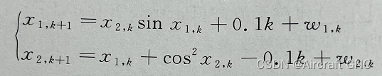
一、状态模型:
二、测量模型:
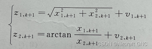
状态方程和测量方程中的噪声均为期望为零的白噪声。
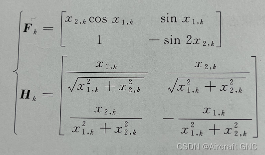
三、状态模型和测量模型的线性化(Jacobian矩阵):
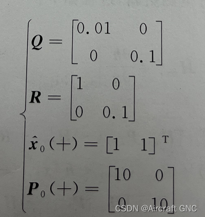
四、状态模型和测量模型的噪声矩阵及初始状态及协方差矩阵:
五、C++ 仿真源码:
EKF.h
#pragma once
#include <fstream>
#include <string>
#include <iostream>
#include <Eigen/Dense>
#include "RandomGenerate.h"
class EKF
{
public:
EKF();
virtual ~EKF();
void Filter();
private:
void Initialize();
void GenerateXreal(int k);
void GenerateZreal();
Eigen::Vector2d Nonlinearf(int k);
Eigen::Matrix2d JacobianMatrixF();
void Prediction(const Eigen::Vector2d& f, const Eigen::Matrix2d& F);
Eigen::Vector2d Nonlinearh();
Eigen::Matrix2d JacobianMatrixH();
void Update(const Eigen::Vector2d& h, const Eigen::Matrix2d& H);
private:
Eigen::Vector2d xpre;
Eigen::Matrix2d Ppre;
Eigen::Matrix2d Q;
Eigen::Matrix2d R;
Eigen::Matrix2d K;
Eigen::Vector2d xest;
Eigen::Matrix2d Pest;
Eigen::Vector2d xreal;
Eigen::Vector2d zreal;
private:
std::string FileName;
std::ofstream outFile;
};
EKF.cpp
#include "EKF.h"
EKF::EKF() : FileName("./FilterEKF.txt"), outFile(FileName, std::ios::out)
{
Initialize();
}
EKF::~EKF()
{
}
void EKF::Initialize()
{
Q << 0.01, 0,
0, 0.1;
R << 1, 0,
0, 0.1;
Pest << 10, 0,
0, 10;
xest << 1, 1;
xreal = xest;
return;
}
void EKF::GenerateXreal(int k)
{
xreal(0) = xreal(1) * sin(xreal(0)) + 0.1 * k + sqrt(Q(0,0)) * getRandom();
xreal(1) = xreal(0) + cos(xreal(1)) * cos(xreal(1)) - 0.1 * k + sqrt(Q(1, 1)) * getRandom();
return;
}
void EKF::GenerateZreal()
{
zreal(0) = xreal.norm() + sqrt(R(0, 0)) * getRandom();;
zreal(1) = atan(xreal(0) / xreal(1)) + sqrt(R(1, 1)) * getRandom();
return;
}
Eigen::Vector2d EKF::Nonlinearf(int k)
{
Eigen::Vector2d f;
f(0) = xest(1) * sin(xest(0)) + 0.1 * k;
f(1) = xest(0) + cos(xest(1)) * cos(xest(1)) - 0.1 * k;
return f;
}
Eigen::Matrix2d EKF::JacobianMatrixF()
{
Eigen::Matrix2d F;
F(0, 0) = xest(1) * cos(xest(0));
F(0, 1) = sin(xest(0));
F(1, 0) = 1.0;
F(1, 1) = -sin(2*xest(1));
return F;
}
void EKF::Prediction(const Eigen::Vector2d &f, const Eigen::Matrix2d &F)
{
xpre = f;
Eigen::Matrix2d Pxx = F * Pest * F.transpose();
Ppre = Pxx + Q;
return;
}
Eigen::Vector2d EKF::Nonlinearh()
{
Eigen::Vector2d h;
h(0) = xpre.norm();
h(1) = atan(xpre(0) / xpre(1));
return h;
}
Eigen::Matrix2d EKF::JacobianMatrixH()
{
Eigen::Matrix2d H;
double a = xpre.norm();
H(0, 0) = xpre(0) / a;
H(0, 1) = xpre(1) / a;
H(1, 0) = xpre(1) / (a * a);
H(1, 1) = -xpre(0) / (a * a);
return H;
}
void EKF::Update(const Eigen::Vector2d& h, const Eigen::Matrix2d& H)
{
Eigen::Matrix2d Pzz = H * Ppre * H.transpose();
Eigen::Matrix2d Pvv = Pzz + R;
Eigen::Matrix2d Pxz = Ppre * H.transpose();
K = Pxz * Pvv.inverse();
xest = xpre + (K * (zreal - h));
Pest = Ppre - (K * Pvv * K.transpose());
return;
}
void EKF::Filter()
{
std::cout << "请输入采样点个数:" << std::endl;
int num;
std::cin >> num;
for (int i = 0; i != num; i++)
{
GenerateXreal(i);
GenerateZreal();
Eigen::Vector2d f = Nonlinearf(i);
Eigen::Matrix2d F = JacobianMatrixF();
Prediction(f, F);
Eigen::Vector2d h = Nonlinearh();
Eigen::Matrix2d H = JacobianMatrixH();
Update(h, H);
outFile << xreal(0) << ", " << xreal(1) << ", " << xest(0) << ", " << xest(1) << ", " << xpre(0) << ", " << xpre(1) << std::endl;
}
return;
}
demo.cpp
#include "UKF.h"
#include "EKF.h"
int main()
{
UKF ukf;
EKF ekf;
ekf.Filter();
system("pause");
return 0;
}
六、仿真结果:
%% 测试 C++ 程序的可行性。
clear;
clc;

%% 读入C++数据
x = dlmread('Filter.txt');
n = length(x(:,1));
t = 1 : n;

%% 状态
figure;
plot(t, x(:,1), '*-');
hold on;
plot(t, x(:,2), 'o-');
legend('real1','real2');
title('状态');
xlabel('时间/s');
grid on;

%% 状态1
figure;
plot(t, x(:,1), 's-', t, x(:,3), 'o-', t, x(:,5),'*-');
legend('real1','est1','pre1');
title('状态1');
xlabel('时间/s');
grid on;

%% 状态2
figure;
plot(t, x(:,2), 's-', t, x(:,4), 'o-', t, x(:,6),'*-');
legend('real2','est2','pre2');
title('状态2');
xlabel('时间/s');
grid on;

%% 状态1误差
figure;
plot(t, x(:,1)-x(:,3), 'o-', t, x(:,1)-x(:,5),'*-');
legend('est1','pre1');
title('状态1误差');
xlabel('时间/s');
grid on;

%% 状态2误差
figure;
plot(t, x(:,2)-x(:,4), 'o-', t, x(:,2)-x(:,6),'*-');
legend('est2','pre2');
title('状态2误差');
xlabel('时间/s');
grid on;


由图 1、图 2 可知,这两个状态虽然是非线性的,但是其总体趋势都呈线性变化,即非线性程度较弱,因此采用 EKF 滤波算法有望实现较好的估计结果;由图 3、图4 来看,EKF 滤波效果较好,对状态 1 和状态 2 均能很好的估计,滤波误差较小,且滤波(估计)的精度比预测的精度高。
本文内容由网友自发贡献,版权归原作者所有,本站不承担相应法律责任。如您发现有涉嫌抄袭侵权的内容,请联系:hwhale#tublm.com(使用前将#替换为@)