小波变换详解
1,简介
We can use the Fourier Transform to transform a signal from its time-domain to its frequency domain. The peaks in the frequency spectrum indicate the most occurring frequencies in the signal. The larger and sharper a peak is, the more prevalent a frequency is in a signal. The location (frequency-value) and height (amplitude) of the peaks in the frequency spectrum then can be used as input for Classifiers like Random Forest or Gradient Boosting.
我们使用傅里叶变换将一个信号从时域转换成频域。频谱中的峰值表示信号中出现次数最多的频率。频谱中锋越大,越尖,表示在信号中出现越普遍。频谱中峰值的位置(频率值)和高度(振幅)可以作为分类器的输入,如随机森林或梯度增强。
The general rule is that this approach of using the Fourier Transform will work very well when the frequency spectrum is stationary. That is, the frequencies present in the signal are not time-dependent; if a signal contains a frequency of x  this frequency should be present equally anywhere in the signal. The more non-stationary/dynamic a signal is, the worse the results will be. That’s too bad, since most of the signals we see in real life are non-stationary in nature. Whether we are talking about ECG signals, the stock market, equipment or sensor data, etc, etc, in real life problems start to get interesting when we are dealing with dynamic systems. A much better approach for analyzing dynamic signals is to use the Wavelet Transform instead of the Fourier Transform.
通常情况下,使用傅里叶变换能够很好的解决问题,这是因为信号不依赖时间变化而变化的;如果信号只包含X ,信号在任何时间段种都是相同的。这样越是非平稳信号,那傅里叶变换的结果越是糟糕。遗憾的是,我们生活种常见的大部分信号都是这种非平稳信号。例如我们常说的ECG信号,股票信息,设备或传感去的数据,等等。在现实生活中,当我们处理动态系统时,问题开始变得有趣。而更有效的方法就是使用小波变换来代替傅里叶变换。
Even though the Wavelet Transform is a very powerful tool for the analysis and classification of time-series and signals, it is unfortunately not known or popular within the field of Data Science. This is partly because you should have some prior knowledge (about signal processing, Fourier Transform and Mathematics) before you can understand the mathematics behind the Wavelet Transform. However, I believe it is also due to the fact that most books, articles and papers are way too theoretical and don’t provide enough practical information on how it should and can be used.
尽管小波变换能够很有效的处理时间相关的分类和信号,但是在数据科学领域并不被人熟知。这是由于在你明白小波变换身后的数学原理前,你需要知道一些前提知识(信号处理,傅里叶变换,数学)。我认为这也是由于大多数书籍、文章和论文都过于理论化,没有提供足够的实用信息来说明如何使用它。
2.1 从傅里叶变换到小波变换
In the previous paper we have seen how the Fourier Transform works. That is, by multiplying a signal with a series of sine-waves with different frequencies we are able to determine which frequencies are present in a signal. If the dot-product between our signal and a sine wave of a certain frequency results in a large amplitude this means that there is a lot of overlap between the two signals, and our signal contains this specific frequency. This is of course because the dot product is a measure of how much two vectors / signals overlap.
从之前的文章种我们知道傅里叶变换是如何工作的。就是通过很多不同频率的正弦波叠加我们能过知道一个信号中存在哪些频率。如果我们的信号和某个频率的正弦波之间的点积导致振幅很大,这意味着这两个信号之间有很多重叠,我们的信号包含这个特定的频率。当然,这是因为点积是衡量两个向量/信号重叠程度的指标。
The thing about the Fourier Transform is that it has a high resolution in the frequency-domain but zero resolution in the time-domain. This means that it can tell us exactly which frequencies are present in a signal, but not at which location in time these frequencies have occurred. This can easily be demonstrated as follows:
傅里叶变换对频域变换有很好的解决方式,但是不能解决时域变换问题。这意味着,它能告诉我们信号包含哪些频段,但是不能告诉我们这个频段是在信号的哪个时间段出现的。下面的例子能够很好的说明问题:
import numpy as np
from matplotlib import pyplot as plt
t_n = 1
N = 100000
T = t_n / N
f_s = 1/T
xa = np.linspace(0, t_n, num=N)
xb = np.linspace(0, t_n/4, num=N/4)
frequencies = [4, 30, 60, 90]
y1a, y1b = np.sin(2*np.pi*frequencies[0]*xa), np.sin(2*np.pi*frequencies[0]*xb)
y2a, y2b = np.sin(2*np.pi*frequencies[1]*xa), np.sin(2*np.pi*frequencies[1]*xb)
y3a, y3b = np.sin(2*np.pi*frequencies[2]*xa), np.sin(2*np.pi*frequencies[2]*xb)
y4a, y4b = np.sin(2*np.pi*frequencies[3]*xa), np.sin(2*np.pi*frequencies[3]*xb)
composite_signal1 = y1a + y2a + y3a + y4a
composite_signal2 = np.concatenate([y1b, y2b, y3b, y4b])
f_values1, fft_values1 = get_fft_values(composite_signal1, T, N, f_s)
f_values2, fft_values2 = get_fft_values(composite_signal2, T, N, f_s)
fig, axarr = plt.subplots(nrows=2, ncols=2, figsize=(12,8))
axarr[0,0].plot(xa, composite_signal1)
axarr[1,0].plot(xa, composite_signal2)
axarr[0,1].plot(f_values1, fft_values1)
axarr[1,1].plot(f_values2, fft_values2)
(...)
plt.tight_layout()
plt.show()
代码未复现
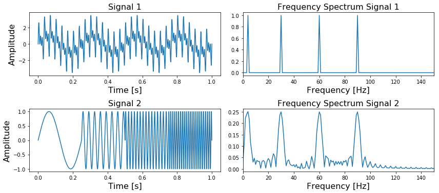
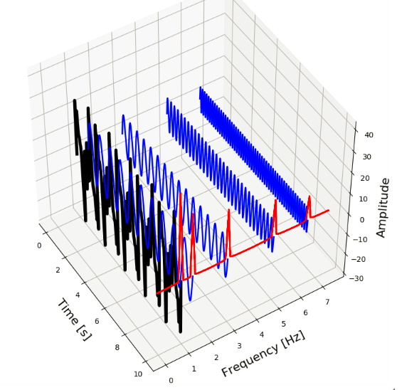
图1,第一行的两个图表示的是一个信号包含4种频率,不因时间的变化而变化。第二行的两个图表示的是信号中的4种频率根据时间依次出现
In Figure 1 we can see at the top left a signal containing four different frequencies ( ,
,  ,
,  and
and  ) which are present at all times and on the right its frequency spectrum. In the bottom figure, we can see the same four frequencies, only the first one is present in the first quarter of the signal, the second one in the second quarter, etc. In addition, on the right side we again see its frequency spectrum.
图1中我们能看到左上角的信号中包含4种不同的频率(, , and ) ,所有频率在这段时间内全部出现,右上角是这个信号的频谱。在下面的两个图中,我们同样能看到这4种频率,但是第一种出现在1/4时间上,之后的频率依次出现。并且我们能在右下面看到这个信号的频谱图。
What is important to note here is that the two frequency spectra contain exactly the same four peaks, so it can not tell us where in the signal these frequencies are present. The Fourier Transform can not distinguish between the first two signals.
值得注意的是两个频谱图都包含了4峰值,但是他们都不能明确表示出在信号的哪个时间段出现的。这就使得傅里叶变换不能区分这个两个信号。
In trying to overcome this problem, scientists have come up with the Short-Time Fourier Transform. In this approach the original signal is splitted into several parts of equal length (which may or may not have an overlap) by using a sliding window before applying the Fourier Transform. The idea is quite simple: if we split our signal into 10 parts, and the Fourier Transform detects a specific frequency in the second part, then we know for sure that this frequency has occurred between  th and
  th of our original signal.
在试图解决这个问题过程种,短时间傅里叶变换出现了。在使用傅里叶变换前对原始信号通过滑动窗口的形式将信号分成几个相同长度。想法很简单:如果我们将信号分割成10份,傅里叶变换找出特殊的信号在第二个部分出现,那么我们就知道这个频段出现在原始信号的 th and th
The main problem with this approach is that you run into the theoretical limits of the Fourier Transform known as the uncertainty principle. The smaller we make the size of the window the more we will know about where a frequency has occurred in the signal, but less about the frequency value itself. The larger we make the size of the window the more we will know about the frequency value and less about the time.
这种方法的主要问题是遇到了傅里叶变换的理论极限即不确定性原理,我们把窗口的大小做得越小,就越能知道信号中某个频率出现在哪里,但是自身的频率值获得的越少。窗口的大小越大,我们对频率值的了解就越多,而对时间的了解就越少。
A better approach for analyzing signals with a dynamical frequency spectrum is the Wavelet Transform. The Wavelet Transform has a high resolution in both the frequency- and the time-domain. It does not only tell us which frequencies are present in a signal, but also at which time these frequencies have occurred. This is accomplished by working with different scales. First we look at the signal with a large scale/window and analyze ‘large’ features and then we look at the signal with smaller scales in order to analyze smaller features.
The time- and frequency resolutions of the different methods are illustrated in Figure 2.
分析这种动态频谱最好的方法就是使用小波变换。小波变换在频域和时域上都有很好的表现。它不仅能够告诉我们在信号种有哪些频率出现,而且能够告诉我们在信号的什么时候出现。这是通过不同的伸缩变换实现的。首先,我们看一个大尺度/窗口的信号,并分析“大”特征,然后我们看一个小尺度的信号,以便分析更小的特征。图2显示了不同方法的时间分辨率和频率分辨率。
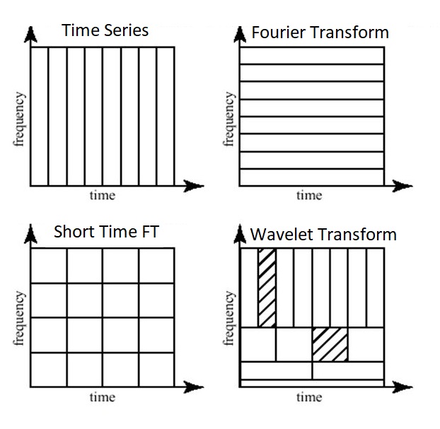
图2,与原始时间序列数据集相比,不同转换的时间和频率分辨率的示意图概述。
In Figure 2 we can see the time and frequency resolutions of the different transformations. The size and orientation of the blocks indicate how small the features are that we can distinguish in the time and frequency domain. The original time-series has a high resolution in the time-domain and zero resolution in the frequency domain. This means that we can distinguish very small features in the time-domain and no features in the frequency domain.
图2我们可以看到不同变换的时间分辨率和频率分辨率。块的大小和方向表明了我们可以在时域和频域区分的特征有多小。原始的时域信号有很高的时域分辨率,频域分辨率为零。这意味着我们能过分辨很小的时域特征但是不能区分频域特征。
Opposite to that is the Fourier Transform, which has a high resolution in the frequency domain and zero resolution in the time-domain.
同样,在频谱种,有很高的频域分辨率但是时域分辨率也是零。
The Short Time Fourier Transform has medium sized resolution in both the frequency and time domain.
短时傅里叶变换在频域和时域均具有中等分辨率。
The Wavelet Transform has:
-
for small frequency values a high resolution in the frequency domain, low resolution in the time- domain,
-
for large frequency values a low resolution in the frequency domain, high resolution in the time domain.
小波变换有:
-
对于小频率值,频域分辨率高,时域分辨率低。
-
对于大频率值,频域分辨率低,时域分辨率高。
In other words, the Wavelet Transforms makes a trade-off; at scales in which time-dependent features are interesting it has a high resolution in the time-domain and at scales in which frequency-dependent features are interesting it has a high resolution in the frequency domain.
And as you can imagine, this is exactly the kind of trade-off we are looking for!
换句话说,小波变换是一种权衡,在与时间相关的特征有趣的尺度上,它在时域具有高分辨率;在与频率相关的特征有趣的尺度上,它在频域具有高分辨率。、
正如你所能想象的,这正是我们正在寻找的一种取舍!
相信大家都看过油画。 对于特别巨幅的油画, 不知道有没有过体会, 油画是只可远观而不可亵玩?
-
当你在足够远的距离观察油画时, 油画所表达的内容是有层次且内容丰富的。
-
当你靠近油画甚至贴在油画上看时, 你只能看到一个个的小色块, 而此时这些小色块此时变成毫无意义的无规则排列。
那我们如何来观看这幅油画呢?
我们假设油画中的每个小色块都对应某一信号中的某个瞬时时间,那么无数个小色块就拼凑成了整幅画, 相当于无数个瞬时时间片段组成了整个信号。
那么,当我们想看看在这个信号的某个时间发生了什么的时候, 我们不得不试图靠近这幅画。
假设一个信号所包含的全部频率信息包含在一副无边无际的油画之中, 辣么, 当你和油画的距离为无穷远的时候你能够毫不费力的看清楚这幅画的全貌,(相当于傅立叶变换,可获得此信号的全部频率信息), 但是你却无法看清楚这幅画的细节(无法得知此信号在某个时刻的瞬时频率)。
当你慢慢走向这幅画的时候(给傅立叶变换加窗), 你走得越近(窗长越短), 细节越清楚(信号的时间分辨率越来越高), 也就是每个小色块都越来越清晰, 但每个色块所包含的信息量(频率信息)也越来越少,这就是著名的海森堡测不准原理(你永远无法得知一个信号之中任一时刻的准确频率信息, 即瞬时频率), 也就是说你永远不可能在距离油画0 cm的位置观测出油画所画的内容。加窗傅立叶变换相当于你选择了一个固定的距离观察这幅油画,当距离近时(窗长减少), 油画的细节更加清楚, 但是油画所表达的信息量随之减少。
这时候就有人提出来了,这个问题还不容易吗? 油画在有的地方细节多,我们就离近一点看嘛(增大变换尺度,增加时间分辨率);有的地方细节少,我们就离得稍微远一点看嘛(减小变化尺度,缩减时间分辨率),这样,在细节和内容的信息量上都能兼顾,能够更全面的欣赏这幅油画,这就是所谓的小波变换啦!
最后总结:
2.2 小波变换是如何工作的
The Fourier Transform uses a series of sine-waves with different frequencies to analyze a signal. That is, a signal is represented through a linear combination of sine-waves. The Wavelet Transform uses a series of functions called wavelets, each with a different scale. The word wavelet means a small wave, and this is exactly what a wavelet is.
傅里叶变换是通过一系列频率不同的正弦波来拟合信号。也就是说,信号是通过正弦波的线性组合来表示的。
小波变换使用一系列称为小波的函数,每个函数具有不同的尺度。小波这个词的意思就是很小的波,的确是这样的。
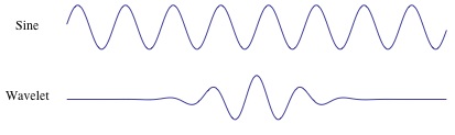
图3,正弦波于小波的不同。正弦波是不限延长的,小波则是在一个时间点上的局域波
In Figure 3 we can see the difference between a sine-wave and a wavelet. The main difference is that the sine-wave is not localized in time (it stretches out from -infinity to +infinity) while a wavelet is localized in time. This allows the wavelet transform to obtain time-information in addition to frequency information.
在图3中,我们能看到正弦波于小波的不同。最主要的不同点是正弦波是一个非时间限制的(是从负无穷到正无穷)波,而小波则是一个时间点上的局域波。这使得小波包含不仅包含频率信息也包含时间信息。
Since the Wavelet is localized in time, we can multiply our signal with the wavelet at different locations in time. We start with the beginning of our signal and slowly move the wavelet towards the end of the signal. This procedure is also known as a convolution. After we have done this for the original (mother) wavelet, we can scale it such that it becomes larger and repeat the process. This process is illustrated in the figure below.
既然小波是在时间上局域的,我们可以叠加不同时间段的小波。我们从信号开始的时间点慢慢想信号结尾移动小波。这个方法也是所说的卷积。在对原始(母)小波做完这些,我们可以改变小波尺寸,使得它变大然后继续上面的操作。这个过程如下图所示。
As we can see in the figure above, the Wavelet transform of an 1-dimensional signal will have two dimensions. This 2-dimensional output of the Wavelet transform is the time-scale representation of the signal in the form of a scaleogram.
由上图可以,经过小波变换信号从1维变成2维。这种小波变换的2维输出是以分布图的形式通过时间尺度变换表示的信号。
So what is this dimension called scale? Since the term frequency is reserved for the Fourier Transform, the wavelet transform is usually expressed in scales instead. That is why the two dimensions of a scaleogram are time and scale. For the ones who find frequencies more intuitive than scales, it is possible to convert scales to pseudo-frequencies with the equation
那么这个scale是什么维度?由于傅里叶变换保留了频率项,所以小波变换通常用尺度来表示。这就是为什么二维分布图有时间和尺度。对于那些认为频率比尺度更直观的人来说,用这个方程可以把尺度转换成伪频率。

where  is the pseudo-frequency,
  is the central frequency of the Mother wavelet and
  is the scaling factor.
其中 是伪频率, 是母小波的中心频率, 是比例因子
We can see that a higher scale-factor (longer wavelet) corresponds with a smaller frequency, so by scaling the wavelet in the time-domain we will analyze smaller frequencies (achieve a higher resolution) in the frequency domain. And vice versa, by using a smaller scale we have more detail in the time-domain. So scales are basically the inverse of the frequency.
我们可以看到越是高的比例(长的小波)对应一个较小的频率,因此在时间维度通过修改小波的比例因子我们可以在频域分析更小的频率(获得更高的分辨率,但是包含的频率信息就少了)。反之一样,通过使用更小的比例因子我们可以在时间维度上获得更多的细节。所以尺度基本上是频率的倒数。
上面的关系也就是说,如果使用更小的比例我们在时域上得到的信息少,在频域上得到的信息多;反之,如果使用更大的比例,在时域上得到的信息多,在频域上得到的信息少。
2.3 小波变换族中的不同类型
Another difference between the Fourier Transform and the Wavelet Transform is that there are many different families (types) of wavelets. The wavelet families differ from each other since for each family a different trade-off has been made in how compact and smooth the wavelet looks like. This means that we can choose a specific wavelet family which fits best with the features we are looking for in our signal.
傅里叶变换和小波变换的另一个不同的地方是小波中有很多不同的族。小波族之间是不同的,因为每个小波族在小波的紧凑性和平滑性方面都做出了不同的权衡。这意味着我们可以选择一个特定的小波族,它最适合我们在信号中寻找的特征。
import pywt
print(pywt.families(short=False))
['Haar', 'Daubechies', 'Symlets', 'Coiflets', 'Biorthogonal', 'Reverse biorthogonal',
'Discrete Meyer (FIR Approximation)', 'Gaussian', 'Mexican hat wavelet', 'Morlet wavelet',
'Complex Gaussian wavelets', 'Shannon wavelets', 'Frequency B-Spline wavelets', 'Complex Morlet wavelets']
Each type of wavelets has a different shape, smoothness and compactness and is useful for a different purpose. Since there are only two mathematical conditions a wavelet has to satisfy it is easy to generate a new type of wavelet.
不同种类的小波有着不同的形状,平滑的和紧密的,用于不同的目的。由于小波只需要满足两个数学条件,因此很容易产生一种新的小波。
The two mathematical conditions are the so-called normalization and orthogonalization constraints:
这两个数学条件就是所谓的归一化约束和正交化约束
A wavelet must have 1) finite energy and 2) zero mean. Finite energy means that it is localized in time and frequency; it is integrable and the inner product between the wavelet and the signal always exists. The admissibility condition implies a wavelet has zero mean in the time-domain, a zero at zero frequency in the time-domain. This is necessary to ensure that it is integrable and the inverse of the wavelet transform can also be calculated.
小波必须有1)有限的能量和2)零均值。
有限能量意味着它在时间和频率上是局域的;它是可积的,小波与信号的内积始终存在。容许条件意味着小波在时域中均值为零,在时域中频率为零时均值为零。这对于保证小波变换的可积性和计算小波变换的逆是必要的。
Furthermore:
-
A wavelet can be orthogonal or non-orthogonal.
-
A wavelet can be bi-orthogonal or not.
-
A wavelet can be symmetric or not.
-
A wavelet can be complex or real. If it is complex, it is usually divided into a real part representing the amplitude and an imaginary part representing the phase.
-
A wavelets is normalized to have unit energy.
此外:
Below we can see a plot with several different families of wavelets. The first row contains four Discrete Wavelets and the second row four Continuous Wavelets.
下面代码中我们看到不同小波族的图像。第一行包含四个离散小波,第二行包含四个连续小波。
import pywt
from matplotlib import pyplot as plt
#print(pywt.families(short=False))
discrete_wavelets = ['db5', 'sym5', 'coif5', 'bior2.4']
continuous_wavelets = ['mexh', 'morl', 'cgau5', 'gaus5']
list_list_wavelets = [discrete_wavelets, continuous_wavelets]
list_funcs = [pywt.Wavelet, pywt.ContinuousWavelet]
fig, axarr = plt.subplots(nrows=2, ncols=4, figsize=(16,8))
for ii, list_wavelets in enumerate(list_list_wavelets):
func = list_funcs[ii]
row_no = ii
for col_no, waveletname in enumerate(list_wavelets):
wavelet = func(waveletname)
family_name = wavelet.family_name
biorthogonal = wavelet.biorthogonal
orthogonal = wavelet.orthogonal
symmetry = wavelet.symmetry
if ii == 0:
_ = wavelet.wavefun()
wavelet_function = _[0]
x_values = _[-1]
else:
wavelet_function, x_values = wavelet.wavefun()
if col_no == 0 and ii == 0:
axarr[row_no, col_no].set_ylabel("Discrete Wavelets", fontsize=16)
if col_no == 0 and ii == 1:
axarr[row_no, col_no].set_ylabel("Continuous Wavelets", fontsize=16)
axarr[row_no, col_no].set_title("{}".format(family_name), fontsize=16)
axarr[row_no, col_no].plot(x_values, wavelet_function)
axarr[row_no, col_no].set_yticks([])
axarr[row_no, col_no].set_yticklabels([])
plt.tight_layout()
plt.show()
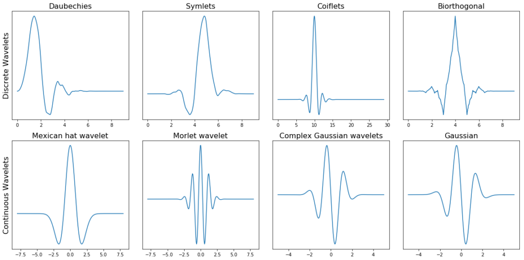
图5 第一行包含四个离散小波,第二行包含四个连续小波。
Within each wavelet family there can be a lot of different wavelet subcategories belonging to that family. You can distinguish the different subcategories of wavelets by the number of coefficients (the number of vanishing moments) and the level of decomposition.
在每个小波族中,可以有许多不同的小波子类别属于这个族。你可以通过系数的数量(消失矩的数量)和分解的级别来区分小波的不同子类别。
This is illustrated below in for the one family of wavelets called ‘Daubechies’.
这是在下面为一个族的小波称为“Daubechies”。
db_wavelets = pywt.wavelist('db')[:5]
print(db_wavelets)
*** ['db1', 'db2', 'db3', 'db4', 'db5']
fig, axarr = plt.subplots(ncols=5, nrows=5, figsize=(20,16))
fig.suptitle('Daubechies family of wavelets', fontsize=16)
for col_no, waveletname in enumerate(db_wavelets):
wavelet = pywt.Wavelet(waveletname)
no_moments = wavelet.vanishing_moments_psi
family_name = wavelet.family_name
for row_no, level in enumerate(range(1,6)):
wavelet_function, scaling_function, x_values = wavelet.wavefun(level = level)
axarr[row_no, col_no].set_title("{} - level {}\n{} vanishing moments\n{} samples".format(
waveletname, level, no_moments, len(x_values)), loc='left')
axarr[row_no, col_no].plot(x_values, wavelet_function, 'bD--')
axarr[row_no, col_no].set_yticks([])
axarr[row_no, col_no].set_yticklabels([])
plt.tight_layout()
plt.subplots_adjust(top=0.9)
plt.show()

图6,多贝西小波族的几个不同的消失时刻和几个层次的细化。
In Figure 6 we can see wavelets of the ‘Daubechies’ family (db) of wavelets. In the first column we can see the Daubechies wavelets of the first order ( db1), in the second column of the second order (db2), up to the fifth order in the fifth column. PyWavelets contains Daubechies wavelets up to order 20 (db20).
图6中我们看到多贝西小波族,第一列中,我们可以看到一阶(db1)的Daubechies小波,在二阶(db2)的第二列中,一直到第五列中的第五阶。小波包含多达20阶(db20)的Daubechies小波。
The number of the order indicates the number of vanishing moments. So db3 has three vanishing moments and db5 has 5 vanishing moment. The number of vanishing moments is related to the approximation order and smoothness of the wavelet. If a wavelet has p vanishing moments, it can approximate polynomials of degree p – 1.
阶数表示消失力矩的个数。所以db3有3个消失力矩db5有5个消失力矩。消去矩的个数与小波的逼近阶数和平滑度有关。如果一个小波有p个消失矩,它可以近似p - 1次多项式
When selecting a wavelet, we can also indicate what the level of decomposition has to be. By default, PyWavelets chooses the maximum level of decomposition possible for the input signal. The maximum level of decomposition (see pywt.dwt_max_level()) depends on the length of the input signal length and the wavelet (more on this later).
在选择小波时,我们还可以指出分解的级别。默认情况下,PyWavelets为输入信号选择可能的最大分解级别。分解的最大级别(参见pywt.dwt_max_level())取决于输入信号长度和小波的长度。
As we can see, as the number of vanishing moments increases, the polynomial degree of the wavelet increases and it becomes smoother. And as the level of decomposition increases, the number of samples this wavelet is expressed in increases.
可以看出,随着消失矩数的增加,小波的多项式阶数增加,小波变得更加平滑。随着分解程度的增加,这个小波的样本数以增加的形式表示。
2.4 连续小波变换与离散小波变换
As we have seen before (Figure 5), the Wavelet Transform comes in two different and distinct flavors; the Continuous and the Discrete Wavelet Transform.
正如我们之前看到的(图5),小波变换有两种不同的风格;连续小波变换和离散小波变换。
Mathematically, a Continuous Wavelet Transform is described by the following equation:
数学上,连续小波变换的表达式为:
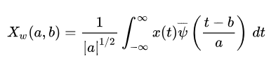
where  is the continuous mother wavelet which gets scaled by a factor of and translated by a factor of
  . The values of the scaling and translation factors are continuous, which means that there can be an infinite amount of wavelets. You can scale the mother wavelet with a factor of 1.3, or 1.31, and 1.311, and 1.3111 etc.
其中为连续母波,a是尺度因子,b为平移因子。尺度因子和平移因子的值是连续的,这意味着可能有无限多的小波。你可以用1.3,或1.31,1.311,和1.3111等因子来缩放母小波。
When we are talking about the Discrete Wavelet Transform, the main difference is that the DWT uses discrete values for the scale and translation factor. The scale factor increases in powers of two, so  and the translation factor increases integer values (
  ).
).
离散小波变换和连续小波变换主要的区别是:离散小波变换对尺度和平移因子使用离散值。缩放因子a aa的幂增加为2(a=1,2,4…… ),平移因子b bb增加整数值(b=1,2,3)。
2.5 离散小波变换的深入:DWT是一组滤波器
In practice, the DWT is always implemented as a filter-bank. This means that it is implemented as a cascade of high-pass and low-pass filters. This is because filter banks are a very efficient way of splitting a signal of into several frequency sub-bands. Below I will try to explain the concept behind the filter-bank in a simple (and probably oversimplified) way. It is necessary in order to understand how the wavelet transform actually works and can be used in practical applications.
在实际应用中,DWT总是被当作滤波器使用。这意味着它被实现为高通滤波器和低通滤波器的级联。这是因为滤波器组是一种非常有效的方法,将一个信号分解成几个子频带。
下面,我将尝试以一种简单(可能过于简化)的方式解释过滤器库背后的概念。了更好地理解小波变换的实际工作原理和在实际应用中应用的必要性。
To apply the DWT on a signal, we start with the smallest scale. As we have seen before, small scales correspond with high frequencies. This means that we first analyze high frequency behavior. At the second stage, the scale increases with a factor of two (the frequency decreases with a factor of two), and we are analyzing behavior around half of the maximum frequency. At the third stage, the scale factor is four and we are analyzing frequency behavior around a quarter of the maximum frequency. And this goes on and on, until we have reached the maximum decomposition level.
要将DWT应用于信号,我们从最小的尺度开始。像我们之前看到的,小尺度的波对应高频。这意味着我们先分析高频行为。在第二阶段,尺度增加一倍(频率减少一倍)。我们在分析最大频率的一半左右的行为。在第三阶段,尺度因子为4,我们正在分析最大频率的四分之一左右的频率行为。这样一直进行下去,直到达到最大分解水平。
What do we mean with maximum decomposition level? To understand this we should also know that at each subsequent stage the number of samples in the signal is reduced with a factor of two. At lower frequency values, you will need less samples to satisfy the Nyquist rate so there is no need to keep the higher number of samples in the signal; it will only cause the transform to be computationally expensive. Due to this downsampling, at some stage in the process the number of samples in our signal will become smaller than the length of the wavelet filter and we will have reached the maximum decomposition level.
最大分解水平是什么意思?为了理解这一点,我们还应该知道,在随后的每个阶段,信号中的样本数量都减少了一倍。在较低的频率值下,您将需要较少的样本来满足奈奎斯特速率,因此无需在信号中保留较高数量的样本;它只会导致转换的计算开销。由于这种下采样,在这个过程的某个阶段,我们的信号中样本的数量会小于小波滤波器的长度,我们将达到最大分解水平。
To give an example, suppose we have a signal with frequencies up to 1000 Hz. In the first stage we split our signal into a low-frequency part and a high-frequency part, i.e. 0-500 Hz and 500-1000 Hz. At the second stage we take the low-frequency part and again split it into two parts: 0-250 Hz and 250-500 Hz.
举个例子,假设我们有一个频率高达1000赫兹的信号。在第一个阶段,我们把信号分成低频部分和高频部分,即0- 500hz和500- 1000hz。在第二阶段,我们取低频部分,再次将其分为两部分:0-250赫兹和250-500赫兹。
At the third stage we split the 0-250 Hz part into a 0-125 Hz part and a 125-250 Hz part. This goes on until we have reached the level of refinement we need or until we run out of samples.
We can easily visualize this idea, by plotting what happens when we apply the DWT on a chirp signal. A chirp signal is a signal with a dynamic frequency spectrum; the frequency spectrum increases with time. The start of the signal contains low frequency values and the end of the signal contains the high frequencies. This makes it easy for us to visualize which part of the frequency spectrum is filtered out by simply looking at the time-axis.
在第三阶段,我们将0-250赫兹的部分分为0-125赫兹的部分和125-250赫兹的部分。
这种情况会一直持续下去,直到我们达到了所需的精化水平,或者直到我们的样本耗尽为止。
我们可以很容易地把这个概念形象化,通过绘制当我们对chirp 信号应用DWT时会发生什么。chirp信号是一种具有动态频谱的信号;频谱随时间而增加。信号的开始包含低频值,信号的结束包含高频值。这使得我们很容易通过简单地观察时间轴来直观地看到频谱的哪一部分被过滤掉了。
import pywt
x = np.linspace(0, 1, num=2048)
chirp_signal = np.sin(250 * np.pi * x**2)
fig, ax = plt.subplots(figsize=(6,1))
ax.set_title("Original Chirp Signal: ")
ax.plot(chirp_signal)
plt.show()
data = chirp_signal
waveletname = 'sym5'
fig, axarr = plt.subplots(nrows=5, ncols=2, figsize=(6,6))
for ii in range(5):
(data, coeff_d) = pywt.dwt(data, waveletname)
axarr[ii, 0].plot(data, 'r')
axarr[ii, 1].plot(coeff_d, 'g')
axarr[ii, 0].set_ylabel("Level {}".format(ii + 1), fontsize=14, rotation=90)
axarr[ii, 0].set_yticklabels([])
if ii == 0:
axarr[ii, 0].set_title("Approximation coefficients", fontsize=14)
axarr[ii, 1].set_title("Detail coefficients", fontsize=14)
axarr[ii, 1].set_yticklabels([])
plt.tight_layout()
plt.show()

图7,应用于chirp信号的sym5小波(1 - 5级)的近似系数和细节系数,从1阶到5阶。在左边,我们可以看到一个示意图表示的高通和低通滤波器应用于信号的每一级。
In Figure 7 we can see our chirp signal, and the DWT applied to it subsequently. There are a few things to notice here:
-
In PyWavelets the DWT is applied with pywt.dwt()
-
The DWT return two sets of coefficients; the approximation coefficients and detail coefficients.
-
The approximation coefficients represent the output of the low pass filter (averaging filter) of the DWT.
-
The detail coefficients represent the output of the high pass filter (difference filter) of the DWT.
-
By applying the DWT again on the approximation coefficients of the previous DWT, we get the wavelet transform of the next level.
-
At each next level, the original signal is also sampled down by a factor of 2.
在图7我们看到chirp信号以及后续的DWT变换。有一下几点需要注意:
-
在小波中,DWT应用pywt.dwt()。
-
DWT返回两组系数;近似系数和细节系数。
-
近似系数表示小波变换的低通滤波器(平均滤波器)的输出。
-
细节系数表示小波变换的高通滤波器(差分滤波器)的输出。
-
通过对上一级小波变换的近似系数进行小波变换,得到下一级小波变换。
-
每下一层,原始信号的采样率也下降2倍。
So now we have seen what it means that the DWT is implemented as a filter bank; At each subsequent level, the approximation coefficients are divided into a coarser low pass and high pass part and the DWT is applied again on the low-pass part.
至此我们看到了DWT作为滤波器是什么意思了。在每一阶,将近似系数分为较粗的低通和高通部分,并对低通部分再次进行小波变换。
As we can see, our original signal is now converted to several signals each corresponding to different frequency bands. Later on we will see how the approximation and detail coefficients at the different frequency sub-bands can be used in applications like removing high frequency noise from signals, compressing signals, or classifying the different types signals.
正如我们所见,我们的原始信号现在被转换成几个信号,每个信号对应不同的频段。稍后,我们将看到在不同频率子带上的近似系数和细节系数如何应用于从信号中去除高频噪声、压缩信号或对不同类型的信号进行分类等应用。
PS: We can also use pywt.wavedec() to immediately calculate the coefficients of a higher level. This functions takes as input the original signal and the level  and returns the one set of approximation coefficients (of the n-th level) and n sets of detail coefficients (1 to n-th level).
备注:我们可以使用pywt.wavedec()函数立即计算出高阶的系数。这个方法需要输入原始信号,阶数并且返回一组近似系数(对应n阶的)和n组细节系数(对应1到n阶)
3.1利用连续小波变换实现状态空间的可视化
So far we have seen what the wavelet transform is, how it is different from the Fourier Transform, what the difference is between the CWT and the DWT, what types of wavelet families there are, what the impact of the order and level of decomposition is on the mother wavelet, and how and why the DWT is implemented as a filter-bank.
至此我们看到了什么是小波变换,它与傅里叶变换的区别是什么,而其中CWT和DWT的区别是什么,小波族的类型都有什么,分解的阶数和层次对母波的影响是什么,小波变换如何以及为什么被实现为一个滤波器库。
We have also seen that the output of a wavelet transform on a 1D signal results in a 2D scaleogram. Such a scaleogram gives us detailed information about the state-space of the system, i.e. it gives us information about the dynamic behavior of the system.
在2D散点图中我们已经看到了小波变换1维信号的输出。这样的比例图为我们提供了关于系统状态空间的详细信息,例如,它给我们展示系统中动态特征的信息
The el-Nino dataset is a time-series dataset used for tracking the El Nino and contains quarterly measurements of the sea surface temperature from 1871 up to 1997. In order to understand the power of a scaleogram, let us visualize it for el-Nino dataset together with the original time-series data and its Fourier Transform.
el-Nino数据集是一个时间序列的数据集用于追踪记录EI Nino现象和包括从1871年至1997年每季度的海面温度测量。为了理解尺度图的威力,让我们将它与原始的时间序列数据及其傅里叶变换一起可视化。
def plot_wavelet(time, signal, scales,
waveletname = 'cmor',
cmap = plt.cm.seismic,
title = 'Wavelet Transform (Power Spectrum) of signal',
ylabel = 'Period (years)',
xlabel = 'Time'):
dt = time[1] - time[0]
[coefficients, frequencies] = pywt.cwt(signal, scales, waveletname, dt)
power = (abs(coefficients)) ** 2
period = 1. / frequencies
levels = [0.0625, 0.125, 0.25, 0.5, 1, 2, 4, 8]
contourlevels = np.log2(levels)
fig, ax = plt.subplots(figsize=(15, 10))
im = ax.contourf(time, np.log2(period), np.log2(power), contourlevels, extend='both',cmap=cmap)
ax.set_title(title, fontsize=20)
ax.set_ylabel(ylabel, fontsize=18)
ax.set_xlabel(xlabel, fontsize=18)
yticks = 2**np.arange(np.ceil(np.log2(period.min())), np.ceil(np.log2(period.max())))
ax.set_yticks(np.log2(yticks))
ax.set_yticklabels(yticks)
ax.invert_yaxis()
ylim = ax.get_ylim()
ax.set_ylim(ylim[0], -1)
cbar_ax = fig.add_axes([0.95, 0.5, 0.03, 0.25])
fig.colorbar(im, cax=cbar_ax, orientation="vertical")
plt.show()
def plot_signal_plus_average(time, signal, average_over = 5):
fig, ax = plt.subplots(figsize=(15, 3))
time_ave, signal_ave = get_ave_values(time, signal, average_over)
ax.plot(time, signal, label='signal')
ax.plot(time_ave, signal_ave, label = 'time average (n={})'.format(5))
ax.set_xlim([time[0], time[-1]])
ax.set_ylabel('Signal Amplitude', fontsize=18)
ax.set_title('Signal + Time Average', fontsize=18)
ax.set_xlabel('Time', fontsize=18)
ax.legend()
plt.show()
def get_fft_values(y_values, T, N, f_s):
f_values = np.linspace(0.0, 1.0/(2.0*T), N//2)
fft_values_ = fft(y_values)
fft_values = 2.0/N * np.abs(fft_values_[0:N//2])
return f_values, fft_values
def plot_fft_plus_power(time, signal):
dt = time[1] - time[0]
N = len(signal)
fs = 1/dt
fig, ax = plt.subplots(figsize=(15, 3))
variance = np.std(signal)**2
f_values, fft_values = get_fft_values(signal, dt, N, fs)
fft_power = variance * abs(fft_values) ** 2 # FFT power spectrum
ax.plot(f_values, fft_values, 'r-', label='Fourier Transform')
ax.plot(f_values, fft_power, 'k--', linewidth=1, label='FFT Power Spectrum')
ax.set_xlabel('Frequency [Hz / year]', fontsize=18)
ax.set_ylabel('Amplitude', fontsize=18)
ax.legend()
plt.show()
dataset = "http://paos.colorado.edu/research/wavelets/wave_idl/sst_nino3.dat"
df_nino = pd.read_table(dataset)
N = df_nino.shape[0]
t0=1871
dt=0.25
time = np.arange(0, N) * dt + t0
signal = df_nino.values.squeeze()
scales = np.arange(1, 128)
plot_signal_plus_average(time, signal)
plot_fft_plus_power(time, signal)
plot_wavelet(time, signal, scales)
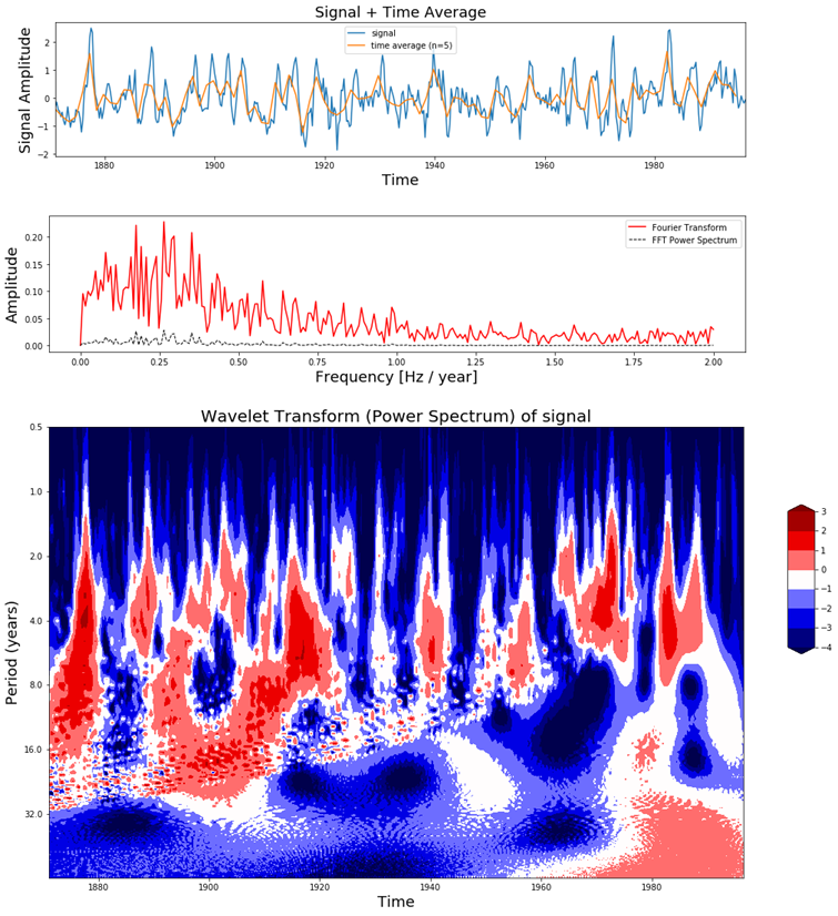
图8,el-Nino数据(最上),经过傅里叶变换后(中间),连续小波变换(底部)
In Figure 8 we can see in the top figure the el-Nino dataset together with its time average, in the middle figure the Fourier Transform and at the bottom figure the scaleogram produced by the Continuous Wavelet Transform.
在图8中,我们能在顶图中看到有时间均值的el-Nino数据集,在中间的图是傅里叶变换的结果,在最底下的图是连续小波变换得到的尺度图。
In the scaleogram we can see that most of the power is concentrated in a 2-8 year period. If we convert this to frequency (T = 1 / f) this corresponds with a frequency of 0.125 – 0.5 Hz. The increase in power can also be seen in the Fourier transform around these frequency values. The main difference is that the wavelet transform also gives us temporal information and the Fourier Transform does not. For example, in the scaleogram we can see that up to 1920 there were many fluctuations, while there were not so much between 1960 – 1990. We can also see that there is a shift from shorter to longer periods as time progresses. This is the kind of dynamic behavior in the signal which can be visualized with the Wavelet Transform but not with the Fourier Transform.
在标度图中我们可以看到大部分的能量集中在2-8年的时间内。如果我们把它转换成频率(T = 1 / f)它对应的频率是0.125 - 0.5 Hz。功率的增加也可以在这些频率值附近的傅里叶变换中看到。主要的区别是小波变换也能给出时间信息,而傅里叶变换不能。例如,在标度图中我们可以看到,在1920年之前有很多波动,而在1960 - 1990年之间没有那么多波动。我们还可以看到,随着时间的推移,从较短的周期向较长的周期转变。这是一种信号的动态行为可以用小波变换来表示但不能用傅里叶变换来表示。
This should already make clear how powerful the wavelet transform can be for machine learning purposes. But to make the story complete, let us also look at how this can be used in combination with a Convolutional Neural Network to classify signals.
应该已经清楚地表明小波变换对于机器学习的作用有多大。但是为了让这篇文章更完整,让我们看看如何结合卷积神经网络来对信号进行分类。
3.2利用连续小波变换和卷积神经网络对信号进行分类
In section 3.1 we have seen that the wavelet transform of a 1D signal results in a 2D scaleogram which contains a lot more information than just the time-series or just the Fourier Transform. We have seen that applied on the el-Nino dataset, it can not only tell us what the period is of the largest oscillations, but also when these oscillations were present and when not.
在3.1节我们已经看到一维信号的小波变换得到二维尺度图,它包含了比时间序列或傅里叶变换多得多的信息。我们看到小波变换在el-Nino数据集上的应用,它不仅能告诉我们最大振荡的周期是多少,还能告诉我们这些振荡是什么时候出现的,什么时候没有。
Such a scaleogram can not only be used to better understand the dynamical behavior of a system, but it can also be used to distinguish different types of signals produced by a system from each other. If you record a signal while you are walking up the stairs or down the stairs, the scaleograms will look different. ECG measurements of people with a healthy heart will have different scaleograms than ECG measurements of people with arrhythmia. Or measurements on a bearing, motor, rotor, ventilator, etc when it is faulty vs when it not faulty. The possibilities are limitless!
这种尺度图不仅能用于更好的理解分析系统的动态特点,而且它还可以用来区分系统产生的不同类型的信号。如果你记录你上楼和下楼的信号,这个尺度图就会不同。正常人的心电图和心律不齐的人的心电图的尺度图会不一样。或测量一个轴承、电机、转子、通风机等,当它有故障时与它没有故障时。可能性是无限的!
So by looking at the scaleograms we can distinguish a broken motor from a working one, a healthy person from a sick one, a person walking up the stairs from a person walking down the stairs, etc etc. But if you are as lazy as me, you probably don’t want to sift through thousands of scaleograms manually. One way to automate this process is to build a Convolutional Neural Network which can automatically detect the class each scaleogram belongs to and classify them accordingly.
所以通过看比例图我们可以区分出一个坏的马达和一个工作的马达,一个健康的人和一个生病的人,一个上楼的人和一个下楼的人等等。但是如果你像我一样懒,您可能不想手动筛选数千个标度图。实现这一过程自动化的一种方法是建立卷积神经网络,该网络可以自动检测每个尺度图所属的类并对其进行分类。
In the next few sections we will load a dataset (containing measurement of people doing six different activities), visualize the scaleograms using the CWT and then use a Convolutional Neural Network to classify these scaleograms.
在接下来的几章里我会加载数据(包含对从事六种不同活动的人的测量),通过CWT可视化尺度图,并且利用卷积神经网络对尺度图进行分类。
3.2.1加载UCI-HAR时序数据集
Let us try to classify an open dataset containing time-series using the scaleograms and a CNN. The Human Activity Recognition Dataset (UCI-HAR) contains sensor measurements of people while they were doing different types of activities, like walking up or down the stairs, laying, standing, walking, etc. There are in total more than 10.000 signals where each signal consists of nine components (x acceleration, y acceleration, z acceleration, x,y,z gyroscope, etc). This is the perfect dataset for us to try our use case of CWT + CNN!
让我们尝试利用尺度图和CNN来对一个开源的时序数据集进行分类。 Human Activity Recognition Dataset (UCI-HAR) 包含通过传感器测量的人类行为,而他们正在做不同类型的活动,如上楼或下楼,躺下,站着,步行等。现有10000多个信号,每个信号由9个分量(x加速度、y加速度、z加速度、x、y、z陀螺仪等)组成。这个是我们利用CWT和CNN最完美的数据集。
UCI-HAR数据集是由30名年龄在19岁至48岁之间的受试者收集的,他们穿着齐腰的智能手机记录运动数据,进行了六项标准活动:
-
Walking
-
Walking Upstairs
-
Walking Downstairs
-
Sitting
-
Standing
-
Laying
移动数据是来自智能手机的x、y和z加速计数据(线性加速度)和陀螺仪数据(角速度),记录频率为50赫兹(即每秒50个数据点)。每个受试者依次执行两次活动,分别将设备置于左手边和右手边。原始数据经过了一些预处理:
After we have downloaded the data, we can load it into a numpy nd-array in the following way:
下载完数据集后,我们可以如下利用numpy将数据集转换为nd-array格式
def read_signals_ucihar(filename):
with open(filename, 'r') as fp:
data = fp.read().splitlines()
data = map(lambda x: x.rstrip().lstrip().split(), data)
data = [list(map(float, line)) for line in data]
return data
def read_labels_ucihar(filename):
with open(filename, 'r') as fp:
activities = fp.read().splitlines()
activities = list(map(int, activities))
return activities
def load_ucihar_data(folder):
train_folder = folder + 'train/InertialSignals/'
test_folder = folder + 'test/InertialSignals/'
labelfile_train = folder + 'train/y_train.txt'
labelfile_test = folder + 'test/y_test.txt'
train_signals, test_signals = [], []
for input_file in os.listdir(train_folder):
signal = read_signals_ucihar(train_folder + input_file)
train_signals.append(signal)
train_signals = np.transpose(np.array(train_signals), (1, 2, 0))
for input_file in os.listdir(test_folder):
signal = read_signals_ucihar(test_folder + input_file)
test_signals.append(signal)
test_signals = np.transpose(np.array(test_signals), (1, 2, 0))
train_labels = read_labels_ucihar(labelfile_train)
test_labels = read_labels_ucihar(labelfile_test)
return train_signals, train_labels, test_signals, test_labels
folder_ucihar = './data/UCI_HAR/'
train_signals_ucihar, train_labels_ucihar, test_signals_ucihar, test_labels_ucihar = load_ucihar_data(folder_ucihar)
The training set contains 7352 signals where each signal has 128 measurement samples and 9 components. The signals from the training set are loaded into a numpy ndarray of size (7352 , 128, 9) and the signals from the test set into one of size (2947 , 128, 9).
训练集包含7352个信号,每个信号包含128个测量样本和9个分量。将训练集转换为格式(7352,128,9)的nd-array,并且测试集转换为(2947 , 128, 9)
Since the signal consists of nine components we have to apply the CWT nine times for each signal. Below we can see the result of the CWT applied on two different signals from the dataset. The left one consist of a signal measured while walking up the stairs and the right one is a signal measured while laying down.
由于信号由9个分量组成,我们必须对每个信号应用9次CWT,下面我们可以看到CWT应用于来自数据集的两个不同信号的结果。左边的是上楼时测量的信号,右边的是躺下时测量的信号。


图9,CWT应用于UCI HAR数据集的两个信号。每个信号有九个不同的分量。在左边我们可以看到上楼时测量到的信号,在右边我们可以看到铺设时测量到的信号。
3.2.2 对数据集机型CWT并且将数据转换成正确的格式
Since each signal has nine components, each signal will also have nine scaleograms. So the next question to ask is, how do we feed this set of nine scaleograms into a Convolutional Neural Network? There are several options we could follow:
因为每个信号有9个分量,所以每个信号也有9个标度图。下一个要问的问题是,我们如何将这9个尺度图输入卷积神经网络?我们有几个选择:
-
Train a CNN for each component separately and combine the results of the nine CNN’s in some sort of an ensembling method. I suspect that this will generally result in a poorer performance since the inter dependencies between the different components are not taken into account.
-
Concatenate the nine different signals into one long signal and apply the CWT on the concatenated signal. This could work but there will be discontinuities at location where two signals are concatenated and this will introduced noise in the scaleogram at the boundary locations of the component signals.
-
Calculate the CWT first and thén concatenate the nine different CWT images into one and feed that into the CNN. This could also work, but here there will also be discontinuities at the boundaries of the CWT images which will feed noise into the CNN. If the CNN is deep enough, it will be able to distinguish between these noisy parts and actually useful parts of the image and choose to ignore the noise. But I still prefer option number four:
-
Place the nine scaleograms on top of each other and create one single image with nine channels. What does this mean? Well, normally an image has either one channel (grayscale image) or three channels (color image), but our CNN can just as easily handle images with nine channels. The way the CNN works remains exactly the same, the only difference is that there will be three times more filters compared to an RGB image.
-
针对每个组件分别训练一个CNN,并以某种综合方法将9个CNN的结果组合起来。我怀疑这通常会导致较差的性能,因为没有考虑到不同组件之间的相互依赖关系。
-
将9个不同的信号串接成一个长信号,并对串接的信号进行CWT处理。这是可行的,但在连接两个信号的位置会有不连续,这将会在分量信号的边界位置的尺度图中引入噪声。
-
首先计算CWT,然后将九幅不同的CWT图像拼接成一幅,并将其输入CNN。这也可以工作,但在这里也会有不连续的CWT图像的边界,这将提供噪声到CNN。如果CNN足够深,它将能够区分这些噪声部分和图像的实际有用部分,并选择忽略噪声。但我还是倾向于选择四:
-
将9个尺度图相互叠加,创建一个带有9个通道的图像。这是什么意思?通常一个图像要么有一个通道(灰度图像)要么有三个通道(彩色图像),但是我们的CNN可以很容易地处理9个通道的图像。CNN的工作方式是完全一样的,唯一的区别是,与RGB图像相比,将有三倍多的过滤器。

图10,我们将使用9个分量中的9个CWT来创建一个用于卷积神经网络输入的9通道图像
Below we can see the Python code on how to apply the CWT on the signals in the dataset, and reformat it in such a way that it can be used as input for our Convolutional Neural Network. The total dataset contains over 10.000 signals, but we will only use 5.000 signals in our training set and 500 signals in our test set.
下面我们会看到Python是如何将数据集中的信号进行CWT的,并且将转换结果转换成下面卷积神经网络输入用的格式。整个数据集包含超过10000个信号,但是我们只用5000个信号用于训练,500个信号用于测试。
scales = range(1,128)
waveletname = 'morl'
train_size = 5000
test_size= 500
train_data_cwt = np.ndarray(shape=(train_size, 127, 127, 9))
for ii in range(0,train_size):
if ii % 1000 == 0:
print(ii)
for jj in range(0,9):
signal = uci_har_signals_train[ii, :, jj]
coeff, freq = pywt.cwt(signal, scales, waveletname, 1)
coeff_ = coeff[:,:127]
train_data_cwt[ii, :, :, jj] = coeff_
test_data_cwt = np.ndarray(shape=(test_size, 127, 127, 9))
for ii in range(0,test_size):
if ii % 100 == 0:
print(ii)
for jj in range(0,9):
signal = uci_har_signals_test[ii, :, jj]
coeff, freq = pywt.cwt(signal, scales, waveletname, 1)
coeff_ = coeff[:,:127]
test_data_cwt[ii, :, :, jj] = coeff_
uci_har_labels_train = list(map(lambda x: int(x) - 1, uci_har_labels_train))
uci_har_labels_test = list(map(lambda x: int(x) - 1, uci_har_labels_test))
x_train = train_data_cwt
y_train = list(uci_har_labels_train[:train_size])
x_test = test_data_cwt
y_test = list(uci_har_labels_test[:test_size])
As you can see above, the CWT of a single signal-component (128 samples) results in an image of 127 by 127 pixels. So the scaleograms coming from the 5000 signals of the training dataset are stored in an numpy ndarray of size (5000, 127, 127, 9) and the scaleograms coming from the 500 test signals are stored in one of size (500, 127, 127, 9).
上面代码所示,单个信号分量(128个样本)的CWT得到127×127像素的图像。因此来自训练数据集的5000个信号的尺度图存储在一个大小为(5000、127、127、9)的numpy nd-array中,来自500个测试信号的尺度图存储在一个大小为(500、127、127、9)的numpy nd-array中。
3.2.3利用CWT进行卷积神经网络训练
Now that we have the data in the right format, we can start with the most interesting part of this section: training the CNN! For this part you will need the keras library, so please install it first.
现在我们已经将数据集转换为正确的格式,我们可以从本节最有趣的部分开始:训练CNN!这节中你将要用到keras库,首先请下载安装这库。
import keras
from keras.layers import Dense, Flatten
from keras.layers import Conv2D, MaxPooling2D
from keras.models import Sequential
from keras.callbacks import History
history = History()

img_x = 127
img_y = 127
img_z = 9
input_shape = (img_x, img_y, img_z)

num_classes = 6
batch_size = 16
num_classes = 7
epochs = 10

x_train = x_train.astype('float32')
x_test = x_test.astype('float32')

y_train = keras.utils.to_categorical(y_train, num_classes)
y_test = keras.utils.to_categorical(y_test, num_classes)


model = Sequential()
model.add(Conv2D(32, kernel_size=(5, 5), strides=(1, 1),
                 activation='relu',
                 input_shape=input_shape))
model.add(MaxPooling2D(pool_size=(2, 2), strides=(2, 2)))
model.add(Conv2D(64, (5, 5), activation='relu'))
model.add(MaxPooling2D(pool_size=(2, 2)))
model.add(Flatten())
model.add(Dense(1000, activation='relu'))
model.add(Dense(num_classes, activation='softmax'))

model.compile(loss=keras.losses.categorical_crossentropy,
              optimizer=keras.optimizers.Adam(),
              metrics=['accuracy'])


model.fit(x_train, y_train,
          batch_size=batch_size,
          epochs=epochs,
          verbose=1,
          validation_data=(x_test, y_test),
          callbacks=[history])

train_score = model.evaluate(x_train, y_train, verbose=0)
print('Train loss: {}, Train accuracy: {}'.format(train_score[0], train_score[1]))
test_score = model.evaluate(x_test, y_test, verbose=0)
print('Test loss: {}, Test accuracy: {}'.format(test_score[0], test_score[1]))

*** Epoch 1/10
*** 5000/5000 [==============================] - 235s 47ms/step - loss: 0.3963 - acc: 0.8876 - val_loss: 0.6006 - val_acc: 0.8780
*** Epoch 2/10
*** 5000/5000 [==============================] - 228s 46ms/step - loss: 0.1939 - acc: 0.9282 - val_loss: 0.3952 - val_acc: 0.8880
*** Epoch 3/10
*** 5000/5000 [==============================] - 224s 45ms/step - loss: 0.1347 - acc: 0.9434 - val_loss: 0.4367 - val_acc: 0.9100
*** Epoch 4/10
*** 5000/5000 [==============================] - 228s 46ms/step - loss: 0.1971 - acc: 0.9334 - val_loss: 0.2662 - val_acc: 0.9320
*** Epoch 5/10
*** 5000/5000 [==============================] - 231s 46ms/step - loss: 0.1134 - acc: 0.9544 - val_loss: 0.2131 - val_acc: 0.9320
*** Epoch 6/10
*** 5000/5000 [==============================] - 230s 46ms/step - loss: 0.1285 - acc: 0.9520 - val_loss: 0.2014 - val_acc: 0.9440
*** Epoch 7/10
*** 5000/5000 [==============================] - 232s 46ms/step - loss: 0.1339 - acc: 0.9532 - val_loss: 0.2884 - val_acc: 0.9300
*** Epoch 8/10
*** 5000/5000 [==============================] - 237s 47ms/step - loss: 0.1503 - acc: 0.9488 - val_loss: 0.3181 - val_acc: 0.9340
*** Epoch 9/10
*** 5000/5000 [==============================] - 250s 50ms/step - loss: 0.1247 - acc: 0.9504 - val_loss: 0.2403 - val_acc: 0.9460
*** Epoch 10/10
*** 5000/5000 [==============================] - 238s 48ms/step - loss: 0.1578 - acc: 0.9508 - val_loss: 0.2133 - val_acc: 0.9300
*** Train loss: 0.11115437872409821, Train accuracy: 0.959
*** Test loss: 0.21326758581399918, Test accuracy: 0.93
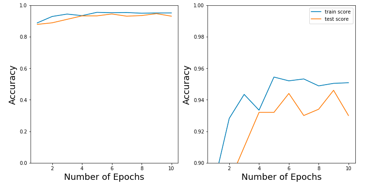
As you can see, combining the Wavelet Transform and a Convolutional Neural Network leads to an awesome and amazing result!
We have an accuracy of 94% on the Activity Recognition dataset. Much higher than you can achieve with any other method. In section 3.5 we will use the Discrete Wavelet Transform instead of Continuous Wavelet Transform to classify the same dataset and achieve similarly amazing results!
正如你所看到的,小波变换和卷积神经网络结合得到了一个很棒的结果!
我们对活动识别数据集的准确率为94%。比任何其他方法都要高得多。
在3.5节中,我们将使用离散小波变换代替连续小波变换对相同的数据集进行分类,得到同样惊人的结果!
3.3用小波分解信号
In Section 2.5 we have seen how the DWT is implemented as a filter-bank which can deconstruct a signal into its frequency sub-bands. In this section, let us see how we can use PyWavelets to deconstruct a signal into its frequency sub-bands and reconstruct the original signal again.
在2.5节,我们已经看到小波变换是如何作为一个滤波器库来实现的,它可以将一个信号分解成它的子频带。这节中,让我们看看如何使用小波将一个信号分解成它的子频带,并重新构造原始信号。
PyWavelets offers two different ways to deconstruct a signal.
-
We can either apply pywt.dwt() on a signal to retrieve the approximation coefficients. Then apply the DWT on the retrieved coefficients to get the second level coefficients and continue this process until you have reached the desired decomposition level.
-
Or we can apply pywt.wavedec() directly and retrieve all of the the detail coefficients up to some level . This functions takes as input the original signal and the level and returns the one set of approximation coefficients (of the n-th level) and n sets of detail coefficients (1 to n-th level).
PyWavelets 提供了2中解析信号的方法。
-
我们可以对信号应用pywt.dwt()来检索近似系数。然后对检索到的系数应用DWT以获得第二级系数,并继续此过程,直到达到所需的分解级别
-
或我们可以应用pywt.wavedec()直接和检索所有的细节系数达到某种程度上n。这个函数作为输入原始信号和n水平并返回一组近似系数(第n个水平)和n组细节系数(1到n级)。
(cA1, cD1) = pywt.dwt(signal, 'db2', 'smooth')
reconstructed_signal = pywt.idwt(cA1, cD1, 'db2', 'smooth')

fig, ax = plt.subplots(figsize=(8,4))
ax.plot(signal, label='signal')
ax.plot(reconstructed_signal, label='reconstructed signal', linestyle='--')
ax.legend(loc='upper left')
plt.show()
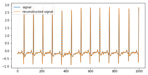
图12,一个信号和重建的信号
Above we have deconstructed a signal into its coefficients and reconstructed it again using the inverse DWT.
面我们将一个信号分解成它的系数,然后再用反DWT对其进行重构。
The second way is to use pywt.wavedec() to deconstruct and reconstruct a signal and it is probably the most simple way if you want to get higher-level coefficients.
第二种方式是使用pywt.wavedec()来解构和重构一个信号,如果您想获得更高级别的系数,这可能是最简单的方法。
coeffs = pywt.wavedec(signal, 'db2', level=8)
reconstructed_signal = pywt.waverec(coeffs, 'db2')

fig, ax = plt.subplots(figsize=(8,4))
ax.plot(signal[:1000], label='signal')
ax.plot(reconstructed_signal[:1000], label='reconstructed signal', linestyle='--')
ax.legend(loc='upper left')
ax.set_title('de- and reconstruction using wavedec()')
plt.show()
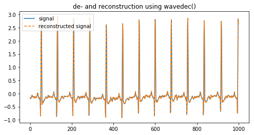
图13,一个信号和其重建的信号
3.4使用DWT去除噪声(高频)噪声
In the previous section we have seen how we can deconstruct a signal into the approximation (low pass) and detail (high pass) coefficients. If we reconstruct the signal using these coefficients we will get the original signal back.
在前一节中,我们已经看到了如何将信号分解为近似(低通)和细节(高通)系数。如果我们用这些系数重建信号,我们将得到原始信号。
But what happens if we reconstruct while we leave out some detail coefficients? Since the detail coefficients represent the high frequency part of the signal, we will simply have filtered out that part of the frequency spectrum. If you have a lot of high-frequency noise in your signal, this one way to filter it out.
如果我们在重建的过程中丢掉一些细节系数会怎么样呢?既然细节系数代表的是信号中的高频部分,我们只需要过滤掉这部分频谱,如果你的信号中有很多高频噪声,这是一种过滤的方法。
Leaving out of the detail coefficients can be done using pywt.threshold(), which removes coefficient values higher than the given threshold.
可以使用pywt.threshold()删除细节系数,它删除了高于给定阈值的系数值。
Lets demonstrate this using NASA’s Femto Bearing Dataset. This is a dataset containing high frequency sensor data regarding accelerated degradation of bearings.
让我们用NASA的飞向轴承数据集来证明这一点。这是一个包含关于轴承加速退化的高频传感器数据集。
DATA_FOLDER = './FEMTO_bearing/Training_set/Bearing1_1/'
filename = 'acc_01210.csv'
df = pd.read_csv(DATA_FOLDER + filename, header=None)
signal = df[4].values

def lowpassfilter(signal, thresh = 0.63, wavelet="db4"):
    thresh = thresh*np.nanmax(signal)
    coeff = pywt.wavedec(signal, wavelet, mode="per" )
    coeff[1:] = (pywt.threshold(i, value=thresh, mode="soft" ) for i in coeff[1:])
    reconstructed_signal = pywt.waverec(coeff, wavelet, mode="per" )
    return reconstructed_signal

fig, ax = plt.subplots(figsize=(12,8))
ax.plot(signal, color="b", alpha=0.5, label='original signal')
rec = lowpassfilter(signal, 0.4)
ax.plot(rec, 'k', label='DWT smoothing}', linewidth=2)
ax.legend()
ax.set_title('Removing High Frequency Noise with DWT', fontsize=18)
ax.set_ylabel('Signal Amplitude', fontsize=16)
ax.set_xlabel('Sample No', fontsize=16)
plt.show()
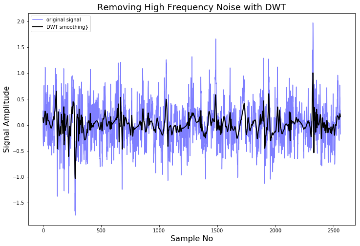
图14,一个高频信号和它的DWT平滑变换图
As we can see, by deconstructing the signal, setting some of the coefficients to zero, and reconstructing it again, we can remove high frequency noise from the signal.
正如我们所看到的,通过解构信号,把一些系数设为零,然后重新构造,我们可以从信号中去除高频噪声。
People who are familiar with signal processing techniques might know there are a lot of different ways to remove noise from a signal. For example, the Scipy library contains a lot of smoothing filters (one of them is the famous Savitzky-Golay filter) and they are much simpler to use. Another method for smoothing a signal is to average it over its time-axis.
熟悉信号处理的人也许知道有很多不同的方法去除信号中的噪声。例如,例如,Scipy库包含许多平滑过滤器(其中之一是著名的Savitzky-Golay过滤器),它们使用起来要简单得多.另一种平滑信号的方法是对其时间轴进行平均。
So why should you use the DWT instead? The advantage of the DWT again comes from the many wavelet shapes there are available. You can choose a wavelet which will have a shape characteristic to the phenomena you expect to see. In this way, less of the phenomena you expect to see will be smoothed out.
那么为什么要使用DWT呢?小波变换的优势又一次来自于现有的许多小波形状。你可以选择一个小波,它将有一个形状特征的现象,你希望看到。这样,你所期望看到的现象就会减少。
3.4使用离散小波变换进行信号分类
In Section 3.2 we have seen how we can use a the CWT and a CNN to classify signals. Of course it is also possible to use the DWT to classify signals. Let us have a look at how this could be done.
在3.2节,我们看到是如何使用连续小波变换和卷积神经网络来对信号进行分类的。当然用离散小波变换来分类信号也是可以的。让我们看一下是如何实现的。
3.5.1离散小波分类的思想
The idea behind DWT signal classification is as follows: The DWT is used to split a signal into different frequency sub-bands, as many as needed or as many as possible. If the different types of signals exhibit different frequency characteristics, this difference in behavior has to be exhibited in one of the frequency sub-bands. So if we generate features from each of the sub-band and use the collection of features as an input for a classifier (Random Forest, Gradient Boosting, Logistic Regression, etc) and train it by using these features, the classifier should be able to distinguish between the different types of signals.
离散小波变换分类思想如下:DWT用于将一个信号分割成不同的子频带,尽可能多的子频带或尽可能多的子频带。如果不同类型的信号表现出不同的频率特性,这种行为上的差异必须表现在一个频率子带中。因此,如果我们从每个子带生成特征,并将这些特征集合作为分类器的输入(Random Forest, Gradient boost, Logistic Regression等),并利用这些特征训练分类器,那么分类器应该能够区分不同类型的信号。
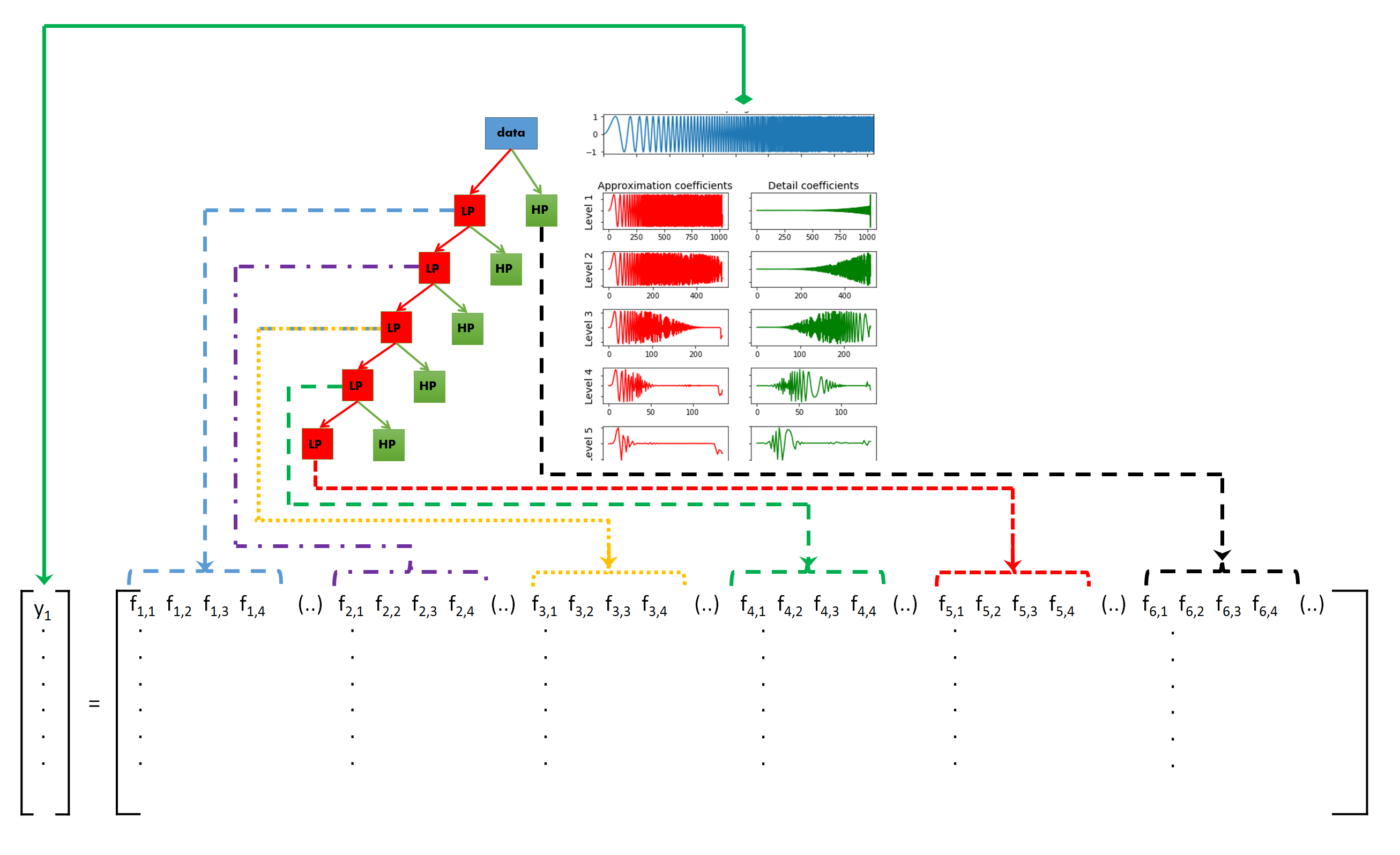
图15,将信号进行离散小波变换,我们可以分解它的频率子带。并从每个子带中提取特征,作为分类器的输入。
3.5.2为每个子带生成特征
So what kind of features can be generated from the set of values for each of the sub-bands? Of course this will highly depend on the type of signal and the application. But in general, below are some features which are most frequently used for signals.
那么,可以从每个子带的值集生成什么样的特性呢?当然,这在很大程度上取决于信号的类型和应用程序。但是一般来说,下面是一些最常用于信号的特性。
-
Auto-regressive model coefficient values
-
(Shannon) Entropy values; entropy values can be taken as a measure of complexity of the signal.
-
Statistical features like:
-
variance
-
standard deviation
-
Mean
-
Median
-
25th percentile value
-
75th percentile value
-
Root Mean Square value; square of the average of the squared amplitude values
-
The mean of the derivative
-
Zero crossing rate, i.e. the number of times a signal crosses y = 0
-
Mean crossing rate, i.e. the number of times a signal crosses y = mean(y)
These are just some ideas you could use to generate the features out of each sub-band. You could use some of the features described here, or you could use all of them. Most classifiers in the scikit-learn package are powerful enough to handle a large number of input features and distinguish between useful ones and non-useful ones. However, I still recommend you think carefully about which feature would be useful for the type of signal you are trying to classify.
这些只是一些想法,你可以用来产生的特点,从每个子带。您可以使用这里描述的一些特性,也可以使用所有这些特性。scikit-learn包中的大多数分类器都足够强大,可以处理大量的输入特性,并区分有用的和无用的。但是,我仍然建议您仔细考虑哪些特性对您要分类的信号类型有用。
Let’s see how this could be done in Python for a few of the above mentioned features:
让我们看看如何在Python中实现上面提到的一些特性:
def calculate_entropy(list_values):
    counter_values = Counter(list_values).most_common()
    probabilities = [elem[1]/len(list_values) for elem in counter_values]
    entropy=scipy.stats.entropy(probabilities)
    return entropy

def calculate_statistics(list_values):
    n5 = np.nanpercentile(list_values, 5)
    n25 = np.nanpercentile(list_values, 25)
    n75 = np.nanpercentile(list_values, 75)
    n95 = np.nanpercentile(list_values, 95)
    median = np.nanpercentile(list_values, 50)
    mean = np.nanmean(list_values)
    std = np.nanstd(list_values)
    var = np.nanvar(list_values)
    rms = np.nanmean(np.sqrt(list_values**2))
    return [n5, n25, n75, n95, median, mean, std, var, rms]

def calculate_crossings(list_values):
    zero_crossing_indices = np.nonzero(np.diff(np.array(list_values) > 0))[0]
    no_zero_crossings = len(zero_crossing_indices)
    mean_crossing_indices = np.nonzero(np.diff(np.array(list_values) > np.nanmean(list_values)))[0]
    no_mean_crossings = len(mean_crossing_indices)
    return [no_zero_crossings, no_mean_crossings]

def get_features(list_values):
    entropy = calculate_entropy(list_values)
    crossings = calculate_crossings(list_values)
    statistics = calculate_statistics(list_values)
    return [entropy] + crossings + statistics
Above we can see
-
a function to calculate the entropy value of an input signal,
-
a function to calculate some statistics like several percentiles, mean, standard deviation, variance, etc,
-
a function to calculate the zero crossings rate and the mean crossings rate,
-
and a function to combine the results of these three functions.
上面代码可以看到:
The final function returns a set of 12 features for any list of values. So if one signal is decomposed into 10 different sub-bands, and we generate features for each sub-band, we will end up with 10*12 = 120 features per signal.
最后一个函数为任何值列表返回一组12个特性。因此,如果将一个信号分解成10个不同的子带,我们为每个子带生成特征,我们将得到每个信号的10*12 = 120个特征。
3.5.3利用特征和scikit-learn分类器对两个ECG数据集进行分类。
So far so good. The next step is to actually use the DWT to decompose the signals in the training set into its sub-bands, calculate the features for each sub-band, use the features to train a classifier and use the classifier to predict the signals in the test-set.
目前为止一切顺利。下一步是实际使用DWT将训练集中的信号分解为子带,计算每个子带的特征,利用特征训练分类器,利用分类器预测测试集中的信号。
We will do this for two time-series datasets:
-
The UCI-HAR dataset which we have already seen in section 3.2. This dataset contains smartphone sensor data of humans while doing different types of activities, like sitting, standing, walking, stair up and stair down.
-
PhysioNet ECG Dataset (download from here) which contains a set of ECG measurements of healthy persons (indicated as Normal sinus rhythm, NSR) and persons with either an arrhythmia (ARR) or a congestive heart failure (CHF). This dataset contains 96 ARR measurements, 36 NSR measurements and 30 CHF measurements.
我们会使用2种时序数据
-
我们已经在3.2节看到过的UCI-HAR数据集。该数据集包含了人类在进行不同类型的活动时的智能手机传感器数据,如坐、站、走、上、下楼梯。
-
PhysioNet ECG数据集,其中包括一组健康人(指正常窦性心律,NSR)和心律失常(ARR)或充血性心力衰竭(CHF)患者的心电图测量。该数据集包含96个ARR测量值、36个NSR测量值和30个CHF测量值。
After we have downloaded both datasets, and placed them in the right folders, the next step is to load them into memory. We have already seen how we can load the UCI-HAR dataset in section 3.2, and below we can see how to load the ECG dataset.
下载了这两个数据集,并将它们放在正确的文件夹中之后,下一步是将它们加载到内存中。我们已经在3.2节中看到了如何加载UCI-HAR数据集,下面我们将看到如何加载ECG数据集。
def load_ecg_data(filename):
    raw_data = sio.loadmat(filename)
    list_signals = raw_data['ECGData'][0][0][0]
    list_labels = list(map(lambda x: x[0][0], raw_data['ECGData'][0][0][1]))
    return list_signals, list_labels


##########

filename = './data/ECG_data/ECGData.mat'
data_ecg, labels_ecg = load_ecg_data(filename)
training_size = int(0.6*len(labels_ecg))
train_data_ecg = data_ecg[:training_size]
test_data_ecg = data_ecg[training_size:]
train_labels_ecg = labels_ecg[:training_size]
test_labels_ecg = labels_ecg[training_size:]
The ECG dataset is saved as a MATLAB file, so we have to use scipy.io.loadmat() to open this file in Python and retrieve its contents (the ECG measurements and the labels) as two separate lists.
The UCI HAR dataset is saved in a lot of .txt files, and after reading the data we save it into an numpy ndarray of size (no of signals, length of signal, no of components) = (10299 , 128, 9)
ECG数据集保存为MATLAB文件,因此我们必须使用scipy.io.loadmat()在Python中打开该文件,并将其内容(ECG测量值和标签)作为两个单独的列表检索。
UCI HAR数据集保存在许多.txt文件中,读取数据后,我们将其保存为numpy ndarray,大小(no of signals, length of signal, no of components) = (10299, 128, 9)
Now let us have a look at how we can get features out of these two datasets.
现在让我们看看如何从这两个数据集中获得特性。
def get_uci_har_features(dataset, labels, waveletname):
    uci_har_features = []
    for signal_no in range(0, len(dataset)):
        features = []
        for signal_comp in range(0,dataset.shape[2]):
            signal = dataset[signal_no, :, signal_comp]
            list_coeff = pywt.wavedec(signal, waveletname)
            for coeff in list_coeff:
                features += get_features(coeff)
        uci_har_features.append(features)
    X = np.array(uci_har_features)
    Y = np.array(labels)
    return X, Y

def get_ecg_features(ecg_data, ecg_labels, waveletname):
    list_features = []
    list_unique_labels = list(set(ecg_labels))
    list_labels = [list_unique_labels.index(elem) for elem in ecg_labels]
    for signal in ecg_data:
        list_coeff = pywt.wavedec(signal, waveletname)
        features = []
        for coeff in list_coeff:
            features += get_features(coeff)
        list_features.append(features)
    return list_features, list_labels

X_train_ecg, Y_train_ecg = get_ecg_features(train_data_ecg, train_labels_ecg, 'db4')
X_test_ecg, Y_test_ecg = get_ecg_features(test_data_ecg, test_labels_ecg, 'db4')

X_train_ucihar, Y_train_ucihar = get_uci_har_features(train_signals_ucihar, train_labels_ucihar, 'rbio3.1')
X_test_ucihar, Y_test_ucihar = get_uci_har_features(test_signals_ucihar, test_labels_ucihar, 'rbio3.1')
What we have done above is to write functions to generate features from the ECG signals and the UCI HAR signals. There is nothing special about these functions and the only reason we are using two seperate functions is because the two datasets are saved in different formats. The ECG dataset is saved in a list, and the UCI HAR dataset is saved in a 3D numpy ndarray.
我们在上面所做的就是编写函数来从ECG信号和UCI HAR信号中生成特征。这些函数没有什么特别之处,我们使用两个单独的函数的唯一原因是这两个数据集以不同的格式保存。ECG数据集保存在列表中,UCI HAR数据集保存在3D numpy ndarray中。
For the ECG dataset we iterate over the list of signals, and for each signal apply the DWT which returns a list of coefficients. For each of these coefficients, i.e. for each of the frequency sub-bands, we calculate the features with the function we have defined previously. The features calculated from all of the different coefficients belonging to one signal are concatenated together, since they belong to the same signal.
对于ECG数据集,我们遍历信号列表,并对每个信号应用DWT, DWT返回系数列表。对于每一个系数,即每一个频率子带,我们用之前定义的函数计算特征。从属于一个信号的所有不同系数计算出来的特征被连接在一起,因为它们属于同一个信号。
The same is done for the UCI HAR dataset. The only difference is that we now have two for-loops since each signal consists of nine components. The features generated from each of the sub-band from each of the signal component are concatenated together.
UCI HAR数据集也是如此。唯一的区别是我们现在有两个for循环,因为每个信号由9个组件组成。将来自每个信号组件的每个子带生成的特性连接在一起。
Now that we have calculated the features for the two datasets, we can use a GradientBoostingClassifier from the scikit-learn library and train it.
现在我们已经计算了这两个数据集的特性,我们可以使用scikit-learn库中的GradientBoostingClassifier并训练它。
cls = GradientBoostingClassifier(n_estimators=2000)
cls.fit(X_train_ecg, Y_train_ecg)
train_score = cls.score(X_train_ecg, Y_train_ecg)
test_score = cls.score(X_test_ecg, Y_test_ecg)
print("Train Score for the ECG dataset is about: {}".format(train_score))
print("Test Score for the ECG dataset is about: {.2f}".format(test_score))

###

cls = GradientBoostingClassifier(n_estimators=2000)
cls.fit(X_train_ucihar, Y_train_ucihar)
train_score = cls.score(X_train_ucihar, Y_train_ucihar)
test_score = cls.score(X_test_ucihar, Y_test_ucihar)
print("Train Score for the UCI-HAR dataset is about: {}".format(train_score))
print("Test Score for the UCI-HAR dataset is about: {.2f}".format(test_score))

*** Train Score for the ECG dataset is about: 1.0
*** Test Score for the ECG dataset is about: 0.93
*** Train Score for the UCI_HAR dataset is about: 1.0
*** Test Score for the UCI-HAR dataset is about: 0.95
As we can see, the results when we use the DWT + Gradient Boosting Classifier are equally amazing!
This approach has an accuracy on the UCI-HAR test set of 95% and an accuracy on the ECG test set of 93%.
正如我们所看到的,当我们使用DWT +梯度增强分类器时,结果同样令人惊讶!
该方法对UCI-HAR检测集的准确率为95%,对ECG检测集的准确率为93%。
3.6小波变换、傅立叶变换与递归神经网络分类精度的比较
So far, we have seen throughout the various blog-posts, how we can classify time-series and signals in different ways. In a previous post we have classified the UCI-HAR dataset using Signal Processing techniques like The Fourier Transform. The accuracy on the test-set was ~91%.
到目前为止,我们已经在各种各样的博客文章中看到,我们如何以不同的方式对时间序列和信号进行分类。之前用傅里叶变换对UCI-HAR数据集进行分类的测试准确率达到91%
In another blog-post, we have classified the same UCI-HAR dataset using Recurrent Neural Networks. The highest achieved accuracy on the test-set was ~86%.
在之前的文章种,同样对UCI-HAR数据集用递归神经网络进行分类,测试最高的测试准确率达到86%
In this blog-post we have achieved an accuracy of ~94% on the test-set with the approach of CWT + CNN and an accuracy of ~95% with the DWT + GradientBoosting approach!
这篇文章种,利用连续小波变换加卷积神经网络达到的准确率是94%,而使用离散小波变换加梯度增强分类器的准确度达到95%
It is clear that the Wavelet Transform has far better results. We could repeat this for other datasets and I suspect there the Wavelet Transform will also outperform.
很显然小波变换能得到更好的结果。我们可以用其他数据集进行测试,可以猜测小波变换也会表现得更好。
What we can also notice is that strangely enough Recurrent Neural Networks perform the worst. Even the approach of simply using the Fourier Transform and then the peaks in the frequency spectrum has an better accuracy than RNN’s.
我们还可以注意到,奇怪的是,递归神经网络表现最差。即使是简单地利用傅里叶变换和频谱峰值的方法,也比RNN具有更高的精度。
This really makes me wonder, what the hell Recurrent Neural Networks are actually good for. It is said that a RNN can learn ‘temporal dependencies in sequential data’. But, if a Fourier Transform can fully describe any signal (no matter its complexity) in terms of the Fourier components, then what more can be learned with respect to ‘temporal dependencies’.
这让我很好奇,递归神经网络到底有什么用。据说RNN可以学习“序列数据中的时间依赖性”。但是,如果傅里叶变换可以用傅里叶分量完全描述任何信号(无论其复杂度如何),那么关于“时间依赖性”我们还能学到什么。
4最后总结
In this blog post we have seen how we can use the Wavelet Transform for the analysis and classification of time-series and signals (and some other stuff). Not many people know how to use the Wavelet Transform, but this is mostly because the theory is not beginner-friendly and the wavelet transform is not readily available in open source programming languages.
在这篇文章中我们看到使用小波变换对时域序列和信号进行分析和分类。并不是很多人知道如何使用小波变换,但这主要是因为该理论对初学者不友好,而且小波变换在开源编程语言中也不容易得到。
Among Data Scientists, the Wavelet Transform remains an undiscovered jewel and I recommend fellow Data Scientists to use it more often. I am very thankful to the contributors of the PyWavelets package who have implemented a large set of Wavelet families and higher level functions for using these wavelets. Thanks to them, Wavelets can now more easily be used by people using the Python programming language.
在数据科学家中,小波变换仍然是一颗未被发现的宝石,我建议其他数据科学家更经常地使用它。我非常感谢PyWavelets包的贡献者,他们使用这些小波实现了一组大的小波族和更高级别的函数。多亏了它们,现在使用Python编程语言的人可以更容易地使用小波。
END