????????????????
欢迎来到本博客
❤️❤️????????
????博主优势:
????????????
博客内容尽量做到思维缜密,逻辑清晰,为了方便读者。
⛳️
座右铭:
行百里者,半于九十。
????????????
本文目录如下:
????????????
目录
????1 概述
????2 运行结果
????3 参考文献
????4 Python代码、数据
????1 概述
文献:

Decadal global temperature variability increases strongly with climate sensitivity | Nature Climate Change
https://www.nature.com/articles/s41558-019-0527-4
https://www.nature.com/articles/s41558-019-0527-4
https://www.nature.com/articles/s41558-019-0527-4
摘要
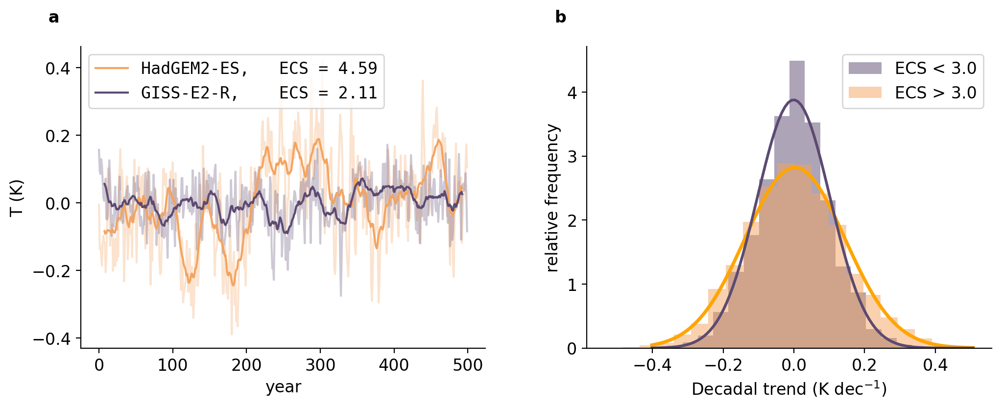
气候相关的风险不仅取决于温室气体的变暖趋势,还取决于这一趋势的变化。然而,对气候变化影响的评估往往集中在全球变暖的最终水平上,偶尔关注全球变暖的速率,而很少关注变化趋势。在这里,我们展示了对温室气体排放更敏感的模型(即更高的平衡气候敏感性(ECS))在数年到数十年时间尺度上也具有更高的温度变化。与直觉相反,高敏感性气候不仅更有可能出现十年尺度的快速变暖,而且更有可能在历史上出现“停滞”时期,而低敏感性气候则更少出现。在历史时期,相对不常见的降温或停滞十年在高ECS世界(ECS=4.5 K)中的可能性是低ECS世界(ECS=1.5 K)的两倍多。由于ECS还影响未受控制的人为强迫未来情景下的背景变暖速率,因此超级变暖十年的可能性——超过二十世纪全球变暖的平均速率十倍以上——对ECS更加敏感。
????
2 运行结果


部分代码:
# The warming probabilities
Z_proj_sup_warm = compute_odds_using_norm_distr(a, b, rate_list2/10, \
warming=True, mn=mn_war)
CS5 = ax5.contour(X, Y, Z_proj_sup_warm.transpose(), 6, colors='C3',\
levels=levels)
CS5.levels = [nf(val)*100 for val in CS5.levels]
ax5.clabel(CS5, CS5.levels, inline=True, fmt=fmt, fontsize=9)
#The cooling probabilities
Z_proj_sup_cool = compute_odds_using_norm_distr(a, b, rate_list2/10, \
warming=False, mn=mn_war)
CS6 = ax5.contour(X, Y, Z_proj_sup_cool.transpose(), 6, colors='c',\
levels=levels)
CS6.levels = [nf(val)*100 for val in CS6.levels]
ax5.clabel(CS6, CS6.levels, inline=True, fmt=fmt, fontsize=9)
ax5.set_xlabel(r'decadal trend (K decade$^{
{-1}}$)', size=12)
ax5.set_ylabel('ECS (K)', size=12)
ax5.set_title("Probability of decadal warming rate under RCP8.5", \
size=12, loc='center')
ax5.plot([anomaly_RCP85, anomaly_RCP85], [2, 4.5], lw=2, c="silver")
return fig, fig_sup, mod_vars
for experiment in ["control", "historical", "projections"]:
#for experiment in ["control"]:
nmods = 16
nfit = 49
#Bayesian, OLS, Bootstrap, Latentx,lognormalpsi, Latentx_quadratic, quadratic
linear_regression_type = 'OLS'
print_each_model = False
filter_models = 0 # filter_models=1 to use model output filtered to HadCRUT4 obs
# Data to consider
if experiment == 'control':
start_yr = 0 # If starting date not permitted; change nyr1 and nyr2
end_yr = 499 # If the end year is 499, one model (GISS) will me omitted
elif experiment == 'historical':
start_yr = 1880 # If starting date not permitted; change nyr1 and nyr2
end_yr = 2012
elif experiment == 'projections':
start_yr = 2000 # If starting date not permitted; change nyr1 and nyr2
end_yr = 2089
elif experiment == 'aroundnow':
start_yr = 1970
end_yr = 2040
stdbetaW15 = []
ECS_best_list = []
ECS_hi_list = []
ECS_lo_list = []
# Detrending options
dtrd = 1
# Length and number of windows
kwind = end_yr-start_yr+1-winlen
# Observational Variables
jvar = 0
var_names = [r'SD$[\beta]$']
jvar_max = len(var_names)
mod_vars_constr = np.zeros((jvar_max, kwind, nmods))
# Define common climatological period
if experiment == 'control':
nyr1 = start_yr
nyr2 = start_yr+30
ensemble = 'control'
elif experiment == 'historical':
nyr1 = 1970 - start_yr
nyr2 = 2000 - start_yr
ensemble = 'hist'
if filter_models > 0: ensemble = 'hist_f'
elif experiment == 'projections':
nyr1 = 2020 - start_yr
nyr2 = 2050 - start_yr
ensemble = 'RCP85'
elif experiment == 'aroundnow':
nyr1 = 1970 - start_yr
nyr2 = 2000 - start_yr
ensemble = 'RCP45'
nyrs = end_yr-start_yr + 1
# ========================================================================
# Get model output
# ========================================================================
N_mods, lambda_mod, ecs_mod, mod_name, mod_lab, dT_mods, yr, _, _ = \
get_CMIP_data(ensemble, nmods, start_yr, end_yr, nyrs, nyr1, nyr2, filter_models, last_n_yrs=True)
# ========================================================================
# Calculate statistics in each window
# ========================================================================
stdT, stdN, ar1T, ratio, mod_vars, end_of_window =\
calculate_major_statistics(dT_mods, N_mods, start_yr, end_yr, yr, jvar_max, dtrd, winlen, nmods)
# ========================================================================
# Calculate key statistics for each model
# ========================================================================
stdN_mod, mod_var, stdT_mod, ar1T_mod, ratio_mod, q2co2, rad_factor = \
calculate_statistics_per_model(stdT, stdN, mod_vars, jvar, ar1T, ratio, ecs_mod, \
mod_lab, mod_name, lambda_mod, print_each_model, nmods)
if experiment == 'control':
print_info_models(ecs_mod, stdN_mod, mod_var, rad_factor)
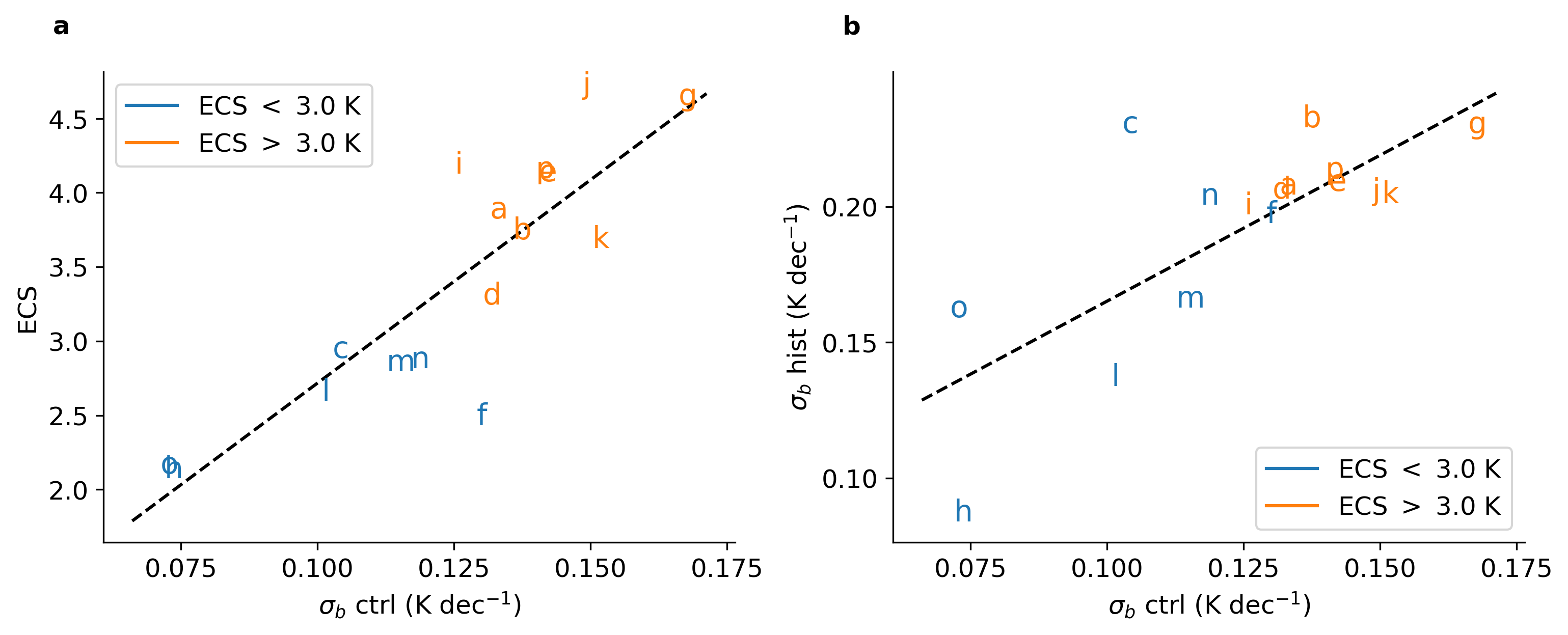
x = mod_var[0:nfit]
if experiment == 'control':
STDB_CTRL = x
ecs = ecs_mod[0:nfit]
xlab = var_names[jvar]
ylab = 'ECS (K)'
corr, dcorr = cross_corr(x, ecs, 0)
print(' ')
print('OLS Correlation of {} and {} in {} = {:.3f} +/- {:.3f}'.format(ylab, \
xlab, experiment, corr, dcorr))
if experiment == 'control':
x_obs = 10 # some fake numbers
dx_obs = 10 # some fake numbers
xfull = mod_var[0:nfit]
yfull = ecs_mod[0:nfit]
a, b, _, _, _, _, _, _, _ = EC_pdf_ECS(xfull, yfull, x_obs, dx_obs, xlab,\
ylab, mod_lab, lambda_mod, nmods, nfit, linear_regression_type, 0)
if experiment == 'control':
# This plots (a) of figure 4
fig_contour_odds, fig_sup, mod_vars_control = fig04_contour(experiment, True, mod_vars, \
fig_contour_odds, fig_sup)
else:
# This plots (c) of figure 4 and maybe also fig ED2a
fig04_contour(experiment, True, mod_vars_control, fig_contour_odds, fig_sup)
if experiment == 'control':
fig_contour_odds, fig_sup, mod_vars_control = fig04_contour(experiment, True, mod_vars, \
fig_contour_odds, fig_sup)
# The scatter part of the figures, so b, d and again b
def scatterandfit(STDB_CTRL, ecs, rate, warming=True):
'''scatterplot of chances getting over certain threshold and ECS,
depending on the background rate'''
if warming is True:
plot_scat_full(ecs, norm(rate, STDB_CTRL).sf(0.07)*100, 'ECS (K)', \
'probability of warming >0.7 K/dec', mod_lab, ecs_mod, 3, ecs_or_lambda='ecs')
OLSfit = sm.OLS(norm(rate, STDB_CTRL).sf(0.07), add_constant(ecs)).fit()
if warming is False:
plot_scat_full(ecs, norm(rate, STDB_CTRL).cdf(0.0)*100, \
'ECS (K)', 'cooling decade chance', mod_lab, ecs_mod, 3, ecs_or_lambda='ecs')
OLSfit = sm.OLS(norm(rate, STDB_CTRL).cdf(0.0), add_constant(ecs)).fit()
rsquared = OLSfit.rsquared
print('rsquared of ECS/anomolous trend X is {:.2f}'.format(rsquared))
return
if experiment == 'historical':
# ax3 assumes that there is a constant background warming, independent of model
ax3 = fig_sup.add_subplot(122)
rate = [anomaly_hist/10] * len(ecs)
plt.sca(ax3)
scatterandfit(STDB_CTRL, ecs, rate, warming=False)
ax3.plot(np.linspace(2.0, 4.5, 100), Z_hist_con[argmin0]*100, lw=2, color='silver')
ax3.set_xlabel('ECS (K)', fontsize=12)
ax3.set_ylabel('Probability (%)', fontsize=12)
ax3.tick_params(axis='both', which='major', labelsize=12)
ax3.set_title(r'Probability of anomaly in trend <-{:.1f} K decade$^{
{-1}}$'.format(anomaly_hist), \
loc='center', size=12)
ax3.spines['right'].set_visible(False) # remove axes top, right
ax3.spines['top'].set_visible(False)
# ax4 assumes a variable background warming, dependent on ECS
ax4 = fig_contour_odds.add_subplot(222)
rate = background_warming('hist')['rate_explained_by_ECS']
rate = background_warming('RCP45', experiment='aroundnow')['rate_explained_by_ECS']
plt.sca(ax4)
scatterandfit(STDB_CTRL, ecs, rate, warming=False)
ax4.plot(np.linspace(2.0, 4.5, 100), Z_hist_sup[argmin0]*100, color='silver', lw=2)
ax4.set_xlabel('ECS (K)', fontsize=12)
ax4.set_ylabel('Probability (%)', fontsize=12)
ax4.tick_params(axis='both', which='major', labelsize=12)
ax4.set_title('Probability cooling under competing processes', size=12, loc='center')
ax4.set_ylim([0.0, 12])
ax4.spines['right'].set_visible(False) # remove axes top, right
ax4.spines['top'].set_visible(False)
????3
参考文献
文章中一些内容引自网络,会注明出处或引用为参考文献,难免有未尽之处,如有不妥,请随时联系删除。

????
4 Python代码、数据
a 小部件