数据处理笔记1:类别不平衡-上采样

from imblearn.pipeline import make_pipeline

model = make_pipeline(

    RandomUnderSampler(random_state=0),

    HistGradientBoostingClassifier(random_state=0)

)

cv_results = cross_validate(

    model, X, y, scoring="balanced_accuracy",

    return_train_score=True, return_estimator=True,

    n_jobs=-1

)

print(

    f"Balanced accuracy mean +/- std. dev.: "

    f"{cv_results['test_score'].mean():.3f} +/- "

    f"{cv_results['test_score'].std():.3f}"

)

activate Liver

pip install -U imbalanced-learn

"""

==============================

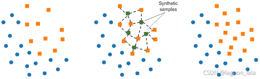
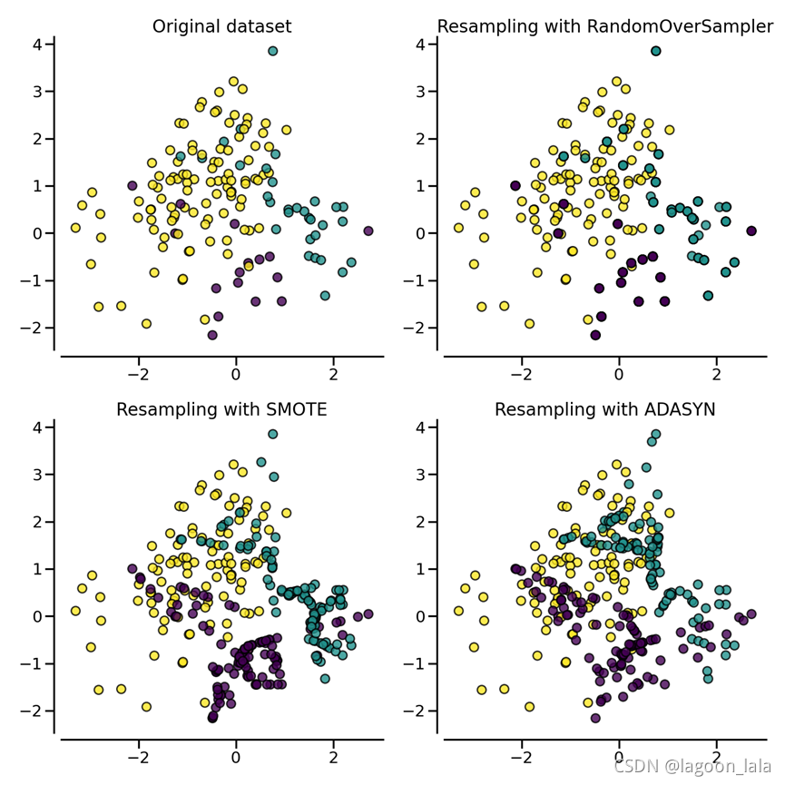
Compare over-sampling samplers

==============================

The following example attends to make a qualitative comparison between the

different over-sampling algorithms available in the imbalanced-learn package.

"""

# Authors: Guillaume Lemaitre <g.lemaitre58@gmail.com>

# License: MIT

# %%

print(__doc__)

import matplotlib.pyplot as plt

import seaborn as sns

sns.set_context("poster")

# %% [markdown]

# The following function will be used to create toy dataset. It uses the

# :func:`~sklearn.datasets.make_classification` from scikit-learn but fixing

# some parameters.

# %%

from sklearn.datasets import make_classification

def create_dataset(

    n_samples=1000,

    weights=(0.01, 0.01, 0.98),

    n_classes=3,

    class_sep=0.8,

    n_clusters=1,

):

    return make_classification(

        n_samples=n_samples,

        n_features=2,

        n_informative=2,

        n_redundant=0,

        n_repeated=0,

        n_classes=n_classes,

        n_clusters_per_class=n_clusters,

        weights=list(weights),

        class_sep=class_sep,

        random_state=0,

    )

# %% [markdown]

# The following function will be used to plot the sample space after resampling

# to illustrate the specificities of an algorithm.

# %%

def plot_resampling(X, y, sampler, ax, title=None):

    X_res, y_res = sampler.fit_resample(X, y)

    ax.scatter(X_res[:, 0], X_res[:, 1], c=y_res, alpha=0.8, edgecolor="k")

    if title is None:

        title = f"Resampling with {sampler.__class__.__name__}"

    ax.set_title(title)

    sns.despine(ax=ax, offset=10)

# %% [markdown]

# The following function will be used to plot the decision function of a

# classifier given some data.

# %%

import numpy as np

def plot_decision_function(X, y, clf, ax, title=None):

    plot_step = 0.02

    x_min, x_max = X[:, 0].min() - 1, X[:, 0].max() + 1

    y_min, y_max = X[:, 1].min() - 1, X[:, 1].max() + 1

    xx, yy = np.meshgrid(

        np.arange(x_min, x_max, plot_step), np.arange(y_min, y_max, plot_step)

    )

    Z = clf.predict(np.c_[xx.ravel(), yy.ravel()])

    Z = Z.reshape(xx.shape)

    ax.contourf(xx, yy, Z, alpha=0.4)

    ax.scatter(X[:, 0], X[:, 1], alpha=0.8, c=y, edgecolor="k")

    if title is not None:

        ax.set_title(title)

# %% [markdown]

# Illustration of the influence of the balancing ratio

# ----------------------------------------------------

#

# We will first illustrate the influence of the balancing ratio on some toy

# data using a logistic regression classifier which is a linear model.

# %%

from sklearn.linear_model import LogisticRegression

clf = LogisticRegression()

# %% [markdown]

# We will fit and show the decision boundary model to illustrate the impact of

# dealing with imbalanced classes.

# %%

fig, axs = plt.subplots(nrows=2, ncols=2, figsize=(15, 12))

weights_arr = (

    (0.01, 0.01, 0.98),

    (0.01, 0.05, 0.94),

    (0.2, 0.1, 0.7),

    (0.33, 0.33, 0.33),

)

for ax, weights in zip(axs.ravel(), weights_arr):

    X, y = create_dataset(n_samples=300, weights=weights)

    clf.fit(X, y)

    plot_decision_function(X, y, clf, ax, title=f"weight={weights}")

    fig.suptitle(f"Decision function of {clf.__class__.__name__}")

fig.tight_layout()

# %% [markdown]

# Greater is the difference between the number of samples in each class, poorer

# are the classification results.

#

# Random over-sampling to balance the data set

# --------------------------------------------

#

# Random over-sampling can be used to repeat some samples and balance the

# number of samples between the dataset. It can be seen that with this trivial

# approach the boundary decision is already less biased toward the majority

# class. The class :class:`~imblearn.over_sampling.RandomOverSampler`

# implements such of a strategy.

# %%

from imblearn.pipeline import make_pipeline

from imblearn.over_sampling import RandomOverSampler

X, y = create_dataset(n_samples=100, weights=(0.05, 0.25, 0.7))

fig, axs = plt.subplots(nrows=1, ncols=2, figsize=(15, 7))

clf.fit(X, y)

plot_decision_function(X, y, clf, axs[0], title="Without resampling")

sampler = RandomOverSampler(random_state=0)

model = make_pipeline(sampler, clf).fit(X, y)

plot_decision_function(X, y, model, axs[1], f"Using {model[0].__class__.__name__}")

fig.suptitle(f"Decision function of {clf.__class__.__name__}")

fig.tight_layout()

# %% [markdown]

# By default, random over-sampling generates a bootstrap. The parameter

# `shrinkage` allows adding a small perturbation to the generated data

# to generate a smoothed bootstrap instead. The plot below shows the difference

# between the two data generation strategies.

# %%

fig, axs = plt.subplots(nrows=1, ncols=2, figsize=(15, 7))

sampler.set_params(shrinkage=None)

plot_resampling(X, y, sampler, ax=axs[0], title="Normal bootstrap")

sampler.set_params(shrinkage=0.3)

plot_resampling(X, y, sampler, ax=axs[1], title="Smoothed bootstrap")

fig.suptitle(f"Resampling with {sampler.__class__.__name__}")

fig.tight_layout()

# %% [markdown]

# It looks like more samples are generated with smoothed bootstrap. This is due

# to the fact that the samples generated are not superimposing with the

# original samples.

#

# More advanced over-sampling using ADASYN and SMOTE

# --------------------------------------------------

#

# Instead of repeating the same samples when over-sampling or perturbating the

# generated bootstrap samples, one can use some specific heuristic instead.

# :class:`~imblearn.over_sampling.ADASYN` and

# :class:`~imblearn.over_sampling.SMOTE` can be used in this case.

# %%

from imblearn import FunctionSampler  # to use a idendity sampler

from imblearn.over_sampling import SMOTE, ADASYN

X, y = create_dataset(n_samples=150, weights=(0.1, 0.2, 0.7))

fig, axs = plt.subplots(nrows=2, ncols=2, figsize=(15, 15))

samplers = [

    FunctionSampler(),

    RandomOverSampler(random_state=0),

    SMOTE(random_state=0),

    ADASYN(random_state=0),

]

for ax, sampler in zip(axs.ravel(), samplers):

    title = "Original dataset" if isinstance(sampler, FunctionSampler) else None

    plot_resampling(X, y, sampler, ax, title=title)

fig.tight_layout()

# %% [markdown]

# The following plot illustrates the difference between

# :class:`~imblearn.over_sampling.ADASYN` and

# :class:`~imblearn.over_sampling.SMOTE`.

# :class:`~imblearn.over_sampling.ADASYN` will focus on the samples which are

# difficult to classify with a nearest-neighbors rule while regular

# :class:`~imblearn.over_sampling.SMOTE` will not make any distinction.

# Therefore, the decision function depending of the algorithm.

X, y = create_dataset(n_samples=150, weights=(0.05, 0.25, 0.7))

fig, axs = plt.subplots(nrows=1, ncols=3, figsize=(20, 6))

models = {

    "Without sampler": clf,

    "ADASYN sampler": make_pipeline(ADASYN(random_state=0), clf),

    "SMOTE sampler": make_pipeline(SMOTE(random_state=0), clf),

}

for ax, (title, model) in zip(axs, models.items()):

    model.fit(X, y)

    plot_decision_function(X, y, model, ax=ax, title=title)

fig.suptitle(f"Decision function using a {clf.__class__.__name__}")

fig.tight_layout()

# %% [markdown]

# Due to those sampling particularities, it can give rise to some specific

# issues as illustrated below.

# %%

X, y = create_dataset(n_samples=5000, weights=(0.01, 0.05, 0.94), class_sep=0.8)

samplers = [SMOTE(random_state=0), ADASYN(random_state=0)]

fig, axs = plt.subplots(nrows=2, ncols=2, figsize=(15, 15))

for ax, sampler in zip(axs, samplers):

    model = make_pipeline(sampler, clf).fit(X, y)

    plot_decision_function(

        X, y, clf, ax[0], title=f"Decision function with {sampler.__class__.__name__}"

    )

    plot_resampling(X, y, sampler, ax[1])

fig.suptitle("Particularities of over-sampling with SMOTE and ADASYN")

fig.tight_layout()

# %% [markdown]

# SMOTE proposes several variants by identifying specific samples to consider

# during the resampling. The borderline version

# (:class:`~imblearn.over_sampling.BorderlineSMOTE`) will detect which point to

# select which are in the border between two classes. The SVM version

# (:class:`~imblearn.over_sampling.SVMSMOTE`) will use the support vectors

# found using an SVM algorithm to create new sample while the KMeans version

# (:class:`~imblearn.over_sampling.KMeansSMOTE`) will make a clustering before

# to generate samples in each cluster independently depending each cluster

# density.

# %%

from imblearn.over_sampling import BorderlineSMOTE, KMeansSMOTE, SVMSMOTE

X, y = create_dataset(n_samples=5000, weights=(0.01, 0.05, 0.94), class_sep=0.8)

fig, axs = plt.subplots(5, 2, figsize=(15, 30))

samplers = [

    SMOTE(random_state=0),

    BorderlineSMOTE(random_state=0, kind="borderline-1"),

    BorderlineSMOTE(random_state=0, kind="borderline-2"),

    KMeansSMOTE(random_state=0),

    SVMSMOTE(random_state=0),

]

for ax, sampler in zip(axs, samplers):

    model = make_pipeline(sampler, clf).fit(X, y)

    plot_decision_function(

        X, y, clf, ax[0], title=f"Decision function for {sampler.__class__.__name__}"

    )

    plot_resampling(X, y, sampler, ax[1])

fig.suptitle("Decision function and resampling using SMOTE variants")

fig.tight_layout()

# %% [markdown]

# When dealing with a mixed of continuous and categorical features,

# :class:`~imblearn.over_sampling.SMOTENC` is the only method which can handle

# this case.

# %%

from collections import Counter

from imblearn.over_sampling import SMOTENC

rng = np.random.RandomState(42)

n_samples = 50

# Create a dataset of a mix of numerical and categorical data

X = np.empty((n_samples, 3), dtype=object)

X[:, 0] = rng.choice(["A", "B", "C"], size=n_samples).astype(object)

X[:, 1] = rng.randn(n_samples)

X[:, 2] = rng.randint(3, size=n_samples)

y = np.array([0] * 20 + [1] * 30)

print("The original imbalanced dataset")

print(sorted(Counter(y).items()))

print()

print("The first and last columns are containing categorical features:")

print(X[:5])

print()

smote_nc = SMOTENC(categorical_features=[0, 2], random_state=0)

X_resampled, y_resampled = smote_nc.fit_resample(X, y)

print("Dataset after resampling:")

print(sorted(Counter(y_resampled).items()))

print()

print("SMOTE-NC will generate categories for the categorical features:")

print(X_resampled[-5:])

print()

# %% [markdown]

# However, if the dataset is composed of only categorical features then one

# should use :class:`~imblearn.over_sampling.SMOTEN`.

# %%

from imblearn.over_sampling import SMOTEN

# Generate only categorical data

X = np.array(["A"] * 10 + ["B"] * 20 + ["C"] * 30, dtype=object).reshape(-1, 1)

y = np.array([0] * 20 + [1] * 40, dtype=np.int32)

print(f"Original class counts: {Counter(y)}")

print()

print(X[:5])

print()

sampler = SMOTEN(random_state=0)

X_res, y_res = sampler.fit_resample(X, y)

print(f"Class counts after resampling {Counter(y_res)}")

print()

print(X_res[-5:])

print()

from sklearn.linear_model import LogisticRegression

clf = LogisticRegression()

from imblearn.pipeline import make_pipeline

from imblearn.over_sampling import RandomOverSampler

X, y = create_dataset(n_samples=100, weights=(0.05, 0.25, 0.7))

fig, axs = plt.subplots(nrows=1, ncols=2, figsize=(15, 7))

clf.fit(X, y)

plot_decision_function(X, y, clf, axs[0], title="Without resampling")

sampler = RandomOverSampler(random_state=0)

model = make_pipeline(sampler, clf).fit(X, y)

plot_decision_function(X, y, model, axs[1], f"Using {model[0].__class__.__name__}")

fig.suptitle(f"Decision function of {clf.__class__.__name__}")

fig.tight_layout()

from collections import Counter

from sklearn.datasets import make_classification

from imblearn.over_sampling import RandomOverSampler

X, y = make_classification(n_classes=2, class_sep=2,

weights=[0.1, 0.9], n_informative=3, n_redundant=1, flip_y=0,

n_features=20, n_clusters_per_class=1, n_samples=1000, random_state=10)

print('Original dataset shape %s' % Counter(y))

Original dataset shape Counter({1: 900, 0: 100})

ros = RandomOverSampler(random_state=42)

X_res, y_res = ros.fit_resample(X, y)

print('Resampled dataset shape %s' % Counter(y_res))

Resampled dataset shape Counter({0: 900, 1: 900})

from imblearn.over_sampling import RandomOverSampler,SMOTE

sm = SMOTE(random_state=42)

X_res, y_res = sm.fit_resample(X, y)

print('Resampled dataset shape %s' % Counter(y_res))

from imblearn.over_sampling import ADASYN

ada = ADASYN(random_state=42)

X_res, y_res = ada.fit_resample(X, y)