up给的教程路线:图像分类→目标检测→…一步步学习用pytorch实现深度学习在cv上的应用,并做笔记整理和总结。
参考内容来自:
up主的b站链接:https://space.bilibili.com/18161609/channel/index
up主将代码和ppt都放在了github:https://github.com/WZMIAOMIAO/deep-learning-for-image-processing
up主的CSDN博客:https://blog.csdn.net/qq_37541097/article/details/103482003
一、卷积神经网络基础与补充
卷积神经网络
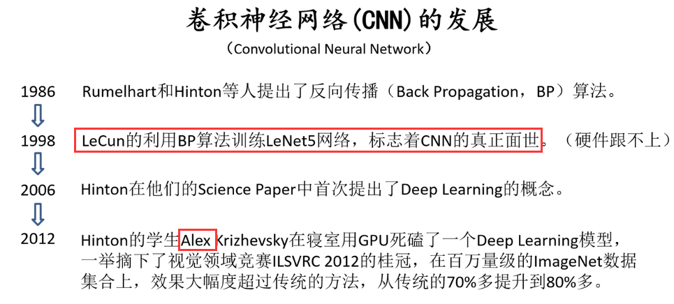
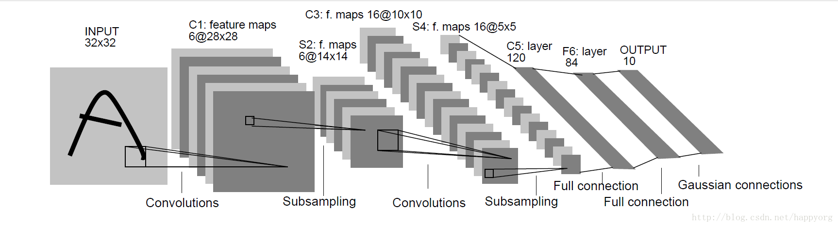
CNN正向传播——以LeNet举例
第一节课主要是通过LeNet网络讲解了CNN中的卷积层、池化层和全连接层的正向传播过程。(包含卷积层的神经网络都可以称为卷积神经网络),由于是基础,就不再赘述。
关于CNN基础可以参考CNN基础
卷积功能
卷积可以提取边缘的特征,比如垂直、水平边缘检测;
如果我们想检测图像的各种边缘特征,而不仅限于垂直边缘和水平边缘,那么 filter 的数值一般需要通过模型训练得到,类似于标准神经网络中的权重 w 一样由反向传播算法迭代求得。CNN的主要目的就是计算出这些 filter 的数值。确定得到了这些 filter 后,CNN浅层网络也就实现了对图片所有边缘特征的检测;
在CNN中,参数数目只由滤波器组决定,数目相对来说要少得多,这是CNN的优势之一。
简单卷积神经网络结构
一个典型的卷积神经网络通常有三层:
- 卷积层:Convolution layers(CONV)
- 池化层:Pooling layers(POOL)
- 全连接层:Fully connected layers(FC)
虽然仅用卷积层也有可能构建出很好的神经网络,但大部分神经网络架构师依然会添加池化层和全连接层。池化层和全连接层比卷积层更容易设计。
关于LeNet网络可以参考LeNet详解
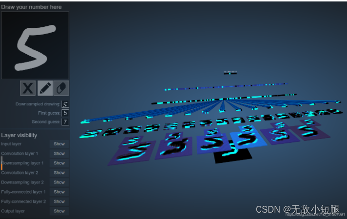
这里推荐一个LeNet的可视化网页,有助于理解(需翻墙)https://www.cs.ryerson.ca/~aharley/vis/conv/
补充1——反向传播中误差的计算:softmax/sigmoid
之前我自己总结过神经网络的反向传播过程,即根据误差的反向传播来更新神经网络的权值。
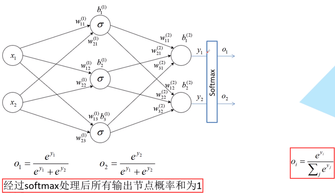
一般是用 交叉熵损失 (Cross Entropy Loss)来计算误差
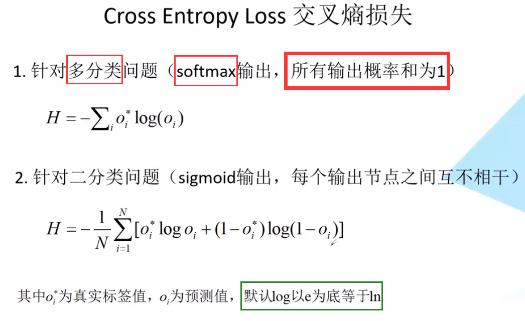
需要注意的是,softmax的所有输出概率和为1,例如进行图像分类时,输入一张图像,是猫的概率为0.3,是狗的概率为0.6,是马的概率为0.1。
补充2——权重的更新
实际应用中,用优化器(optimazer)来优化梯度的求解过程,即让网络得到更快的收敛:
- SGD优化器(Stochastic Gradient Descent 随机梯度下降)
缺点:1. 易受样本噪声影响;2. 可能陷入局部最优解
改进:SGD+Momentum优化器
缺点:学习率下降的太快,可能还没收敛就停止训练
改进:RMSProp优化器:控制下降速度
详情可参考机器学习:各种优化器Optimizer的总结与比较
附图:几种优化器下降的可视化比较
二、LeNet网络——pytorch官方demo分类器
参考:
-
哔哩哔哩:pytorch官方demo(Lenet)
-
pytorch官网demo(中文版戳这里)
-
pytorch中的卷积操作详解
1.demo流程
- model.py ——定义LeNet网络模型
- train.py ——加载数据集并训练,训练集计算loss,测试集计算accuracy,保存训练好的网络参数
- predict.py——得到训练好的网络参数后,用自己找的图像进行分类测试
1.model.py
#模型
# 使用torch.nn包来构建神经网络.
import torch.nn as nn
import torch.nn.functional as F
class LeNet(nn.Module): # 继承于nn.Module这个父类
def __init__(self): # 初始化网络结构
super(LeNet, self).__init__() # 多继承需用到super函数
self.conv1 = nn.Conv2d(3, 16, 5)
self.pool1 = nn.MaxPool2d(2, 2)
self.conv2 = nn.Conv2d(16, 32, 5)
self.pool2 = nn.MaxPool2d(2, 2)
self.fc1 = nn.Linear(32*5*5, 120)
self.fc2 = nn.Linear(120, 84)
self.fc3 = nn.Linear(84, 10)
def forward(self, x): # 正向传播过程
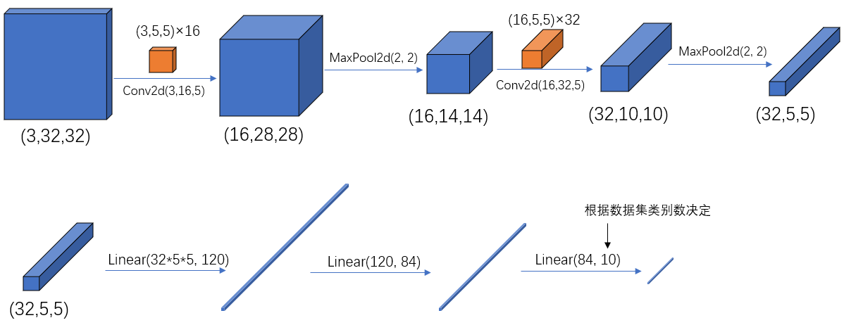
x = F.relu(self.conv1(x)) # input(3, 32, 32) output(16, 28, 28)
x = self.pool1(x) # output(16, 14, 14)
x = F.relu(self.conv2(x)) # output(32, 10, 10)
x = self.pool2(x) # output(32, 5, 5)
x = x.view(-1, 32*5*5) # output(32*5*5)
x = F.relu(self.fc1(x)) # output(120)
x = F.relu(self.fc2(x)) # output(84)
x = self.fc3(x) # output(10)
return x
需注意:
- pytorch 中 tensor(也就是输入输出层)的 通道排序为:
[batch, channel, height, width]
- pytorch中的卷积、池化、输入输出层中参数的含义与位置,可配合下图一起使用:
1.1 卷积 Conv2d
pytorch中函数是
torch.nn.Conv2d(in_channels, out_channels, kernel_size, stride=1, padding=0, dilation=1, groups=1, bias=True, padding_mode='zeros')
一般使用时关注以下几个参数即可:
- in_channels:输入特征矩阵的深度。如输入一张RGB彩色图像,那in_channels=3
- out_channels:输入特征矩阵的深度。也等于卷积核的个数,使用n个卷积核输出的特征矩阵深度就是n
- kernel_size:卷积核的尺寸。可以是int类型,如3 代表卷积核的height=width=3,也可以是tuple类型如(3, 5)代表卷积核的height=3,width=5
- stride:卷积核的步长。默认为1,和kernel_size一样输入可以是int型,也可以是tuple类型
- padding:补零操作,默认为0。可以为int型如1即补一圈0,如果输入为tuple型如(2, 1) 代表在上下补2行,左右补1列。
我们用 s表示stride长度,p表示padding长度,如果原始图片尺寸为 n × n ,filter尺寸为 f × f,则卷积后的图片尺寸为:
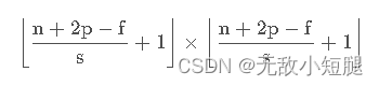
注:商不是整数的情况下,向下取整,上式中的 ⌊ . . . ⌋ 表示向下取整。
1.2 池化 MaxPool2d
最大池化(MaxPool2d)在 pytorch 中对应的函数是:
MaxPool2d(kernel_size, stride)
1.3 Tensor的展平:view()
注意到,在经过第二个池化层后,数据还是一个三维的Tensor (32, 5, 5),需要先经过展平后(32*5*5)再传到全连接层:
  x = self.pool2(x)            # output(32, 5, 5)
  x = x.view(-1, 32*5*5)       # output(32*5*5)
  x = F.relu(self.fc1(x))      # output(120)
1.4 全连接 Linear
全连接( Linear)在 pytorch 中对应的函数是:
Linear(in_features, out_features, bias=True)
2. train.py
2.1数据集预处理、加载
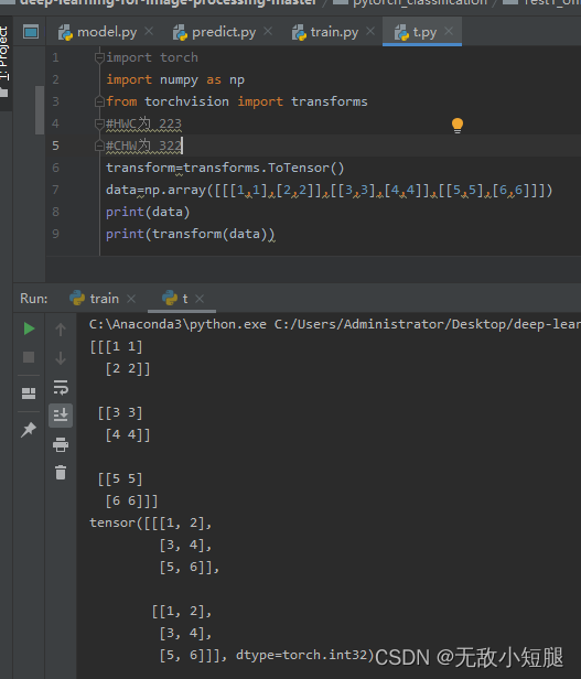
- transform将HWC [0,255]转化为CHW [0,1];对于HWC可以想象取W个H,然后再取C个HW;对于CHW可以想象取H个W,再取C个HW
import torch
import torchvision
import torch.nn as nn
from model import LeNet
import torch.optim as optim
import torchvision.transforms as transforms
transform = transforms.Compose(
        [transforms.ToTensor(),
         transforms.Normalize((0.5, 0.5, 0.5), (0.5, 0.5, 0.5))])

    # 50000张训练图片
    # 第一次使用时要将download设置为True才会自动去下载数据集
    train_set = torchvision.datasets.CIFAR10(root='./data', train=True,
                                             download=False, transform=transform)
    train_loader = torch.utils.data.DataLoader(train_set, batch_size=36,
                                               shuffle=True, num_workers=0)

    # 10000张验证图片
    # 第一次使用时要将download设置为True才会自动去下载数据集
    val_set = torchvision.datasets.CIFAR10(root='./data', train=False,
                                           download=False, transform=transform)
    val_loader = torch.utils.data.DataLoader(val_set, batch_size=5000,
                                             shuffle=False, num_workers=0)
    val_data_iter = iter(val_loader)
    val_image, val_label = next(val_data_iter)

    # classes = ('plane', 'car', 'bird', 'cat',
    #            'deer', 'dog', 'frog', 'horse', 'ship', 'truck')
2.2训练
| 名词 |
定义 |
| epoch |
对训练集的全部数据进行一次完整的训练,称为 一次 epoch |
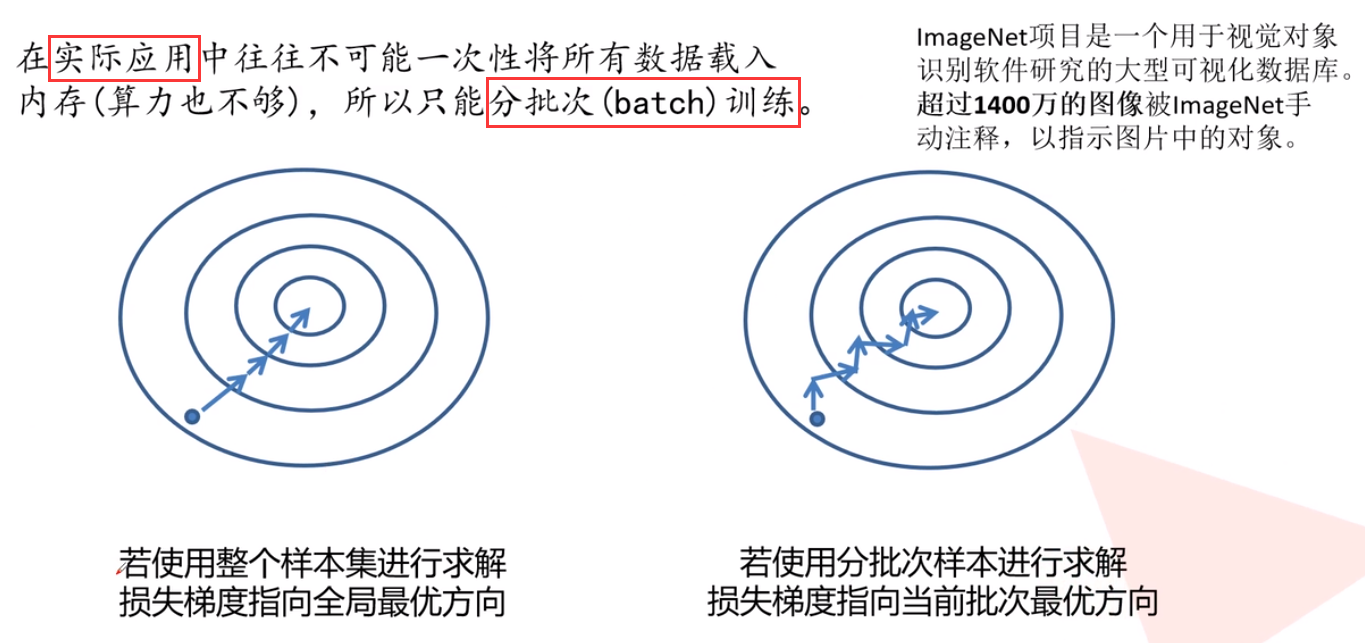
| batch |
由于硬件算力有限,实际训练时将训练集分成多个批次训练,每批数据的大小为 batch_size |
| iteration 或 step |
对一个batch的数据训练的过程称为 一个 iteration 或 step |
net = LeNet()						  				# 定义训练的网络模型
loss_function = nn.CrossEntropyLoss() 				# 定义损失函数为交叉熵损失函数
optimizer = optim.Adam(net.parameters(), lr=0.001)  # 定义优化器(训练参数,学习率)

for epoch in range(5):  # 一个epoch即对整个训练集进行一次训练
    running_loss = 0.0
    time_start = time.perf_counter()

    for step, data in enumerate(train_loader, start=0):   # 遍历训练集,step从0开始计算
        inputs, labels = data 	# 获取训练集的图像和标签
        optimizer.zero_grad()   # 清除历史梯度

        # forward + backward + optimize
        outputs = net(inputs)  				  # 正向传播
        loss = loss_function(outputs, labels) # 计算损失
        loss.backward() 					  # 反向传播
        optimizer.step() 					  # 优化器更新参数

        # 打印耗时、损失、准确率等数据
        running_loss += loss.item()
        if step % 1000 == 999:    # print every 1000 mini-batches,每1000步打印一次
            with torch.no_grad(): # 在以下步骤中(验证过程中)不用计算每个节点的损失梯度,防止内存占用
                outputs = net(test_image) 				 # 测试集传入网络(test_batch_size=10000),output维度为[10000,10]
                predict_y = torch.max(outputs, dim=1)[1] # 以output中值最大位置对应的索引(标签)作为预测输出
                accuracy = (predict_y == test_label).sum().item() / test_label.size(0)

                print('[%d, %5d] train_loss: %.3f  test_accuracy: %.3f' %  # 打印epoch,step,loss,accuracy
                      (epoch + 1, step + 1, running_loss / 500, accuracy))

                print('%f s' % (time.perf_counter() - time_start))        # 打印耗时
                running_loss = 0.0

print('Finished Training')

# 保存训练得到的参数
save_path = './Lenet.pth'
torch.save(net.state_dict(), save_path)
2.3使用GPU训练
device = torch.device("cuda" if torch.cuda.is_available() else "cpu")
print(device)
数据集和网络需要.to(device)
3.predict.py
3.1重要函数
- x.view():展平
- torch.unsqueeze():增加维度
- torch.max():找最大值以及下标
# 导入包
import torch
import torchvision.transforms as transforms
from PIL import Image
from model import LeNet

# 数据预处理需要和训练一样
transform = transforms.Compose(
    [transforms.Resize((32, 32)), # 首先需resize成跟训练集图像一样的大小
     transforms.ToTensor(),
     transforms.Normalize((0.5, 0.5, 0.5), (0.5, 0.5, 0.5))])

# 导入要测试的图像(自己找的,不在数据集中),放在源文件目录下
im = Image.open('horse.jpg')
im = transform(im)  # [C, H, W]
im = torch.unsqueeze(im, dim=0)  # 对数据增加一个新维度,因为tensor的参数是[batch, channel, height, width]

# 实例化网络,加载训练好的模型参数
net = LeNet()#创建一个参数随机的模型
net.load_state_dict(torch.load('Lenet.pth'))#训练时保存的只有权重,所以加载只加载权重

# 预测
classes = ('plane', 'car', 'bird', 'cat',
           'deer', 'dog', 'frog', 'horse', 'ship', 'truck')
with torch.no_grad():
    outputs = net(im)
    predict = torch.max(outputs, dim=1)[1].data.numpy() #torch.max返回两值,第一个是值第二个是最大值下标
print(classes[int(predict)])
其实预测结果也可以用 softmax 表示,输出10个概率:
with torch.no_grad():
    outputs = net(im)
    predict = torch.softmax(outputs, dim=1)
print(predict)
三、搭建AlexNet训练分类数据集
学习资料:
- AlexNet网络结构详解与花分类数据集下载
- 使用pytorch搭建AlexNet并训练花分类数据集
1.准备、划分、预处理、加载数据集
注意:
-
ImageFolder函数
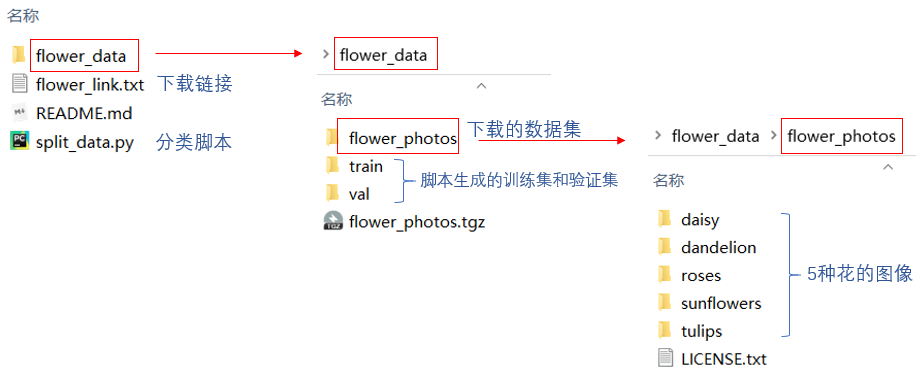
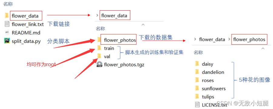
1.1下载数据集
http://download.tensorflow.org/example_images/flower_photos.tgz
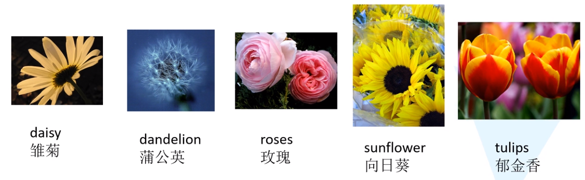
包含 5 中类型的花,每种类型有600~900张图像不等。
1.2 划分数据集——训练集以及测试集
将数据集进行split的脚本
1.3 预处理数据集
- 需要注意的是,对训练集的预处理,多了随机裁剪和水平翻转这两个步骤。可以起到扩充数据集的作用,增强模型泛化能力
- 针对训练集以及测试集不同的预处理
 data_transform = {
        "train": transforms.Compose([transforms.RandomResizedCrop(224),
                                     transforms.RandomHorizontalFlip(),
                                     transforms.ToTensor(),
                                     transforms.Normalize((0.5, 0.5, 0.5), (0.5, 0.5, 0.5))]),
        "val": transforms.Compose([transforms.Resize((224, 224)),  # cannot 224, must (224, 224)
                                   transforms.ToTensor(),
                                   transforms.Normalize((0.5, 0.5, 0.5), (0.5, 0.5, 0.5))])}
1.4导入、加载训练集
- 上篇LetNet网络搭建中是使用的
torchvision.datasets.CIFAR10和torch.utils.data.DataLoader()来导入和加载数据集。
-
花分类数据集 并不在 pytorch 的
torchvision.datasets中,因此需要用到datasets.ImageFolder(root,transform)来导入。root代表最大文件夹的路径,root下面有多个文件夹,文件夹名是label,文件夹里面是label对应的图片。
-
ImageFolder()返回的对象是一个包含数据集所有图像及对应标签构成的二维元组容器,支持索引和迭代,可作为torch.utils.data.DataLoader的输入。
# 导入包
import torch
import torch.nn as nn
from torchvision import transforms, datasets, utils


# 使用GPU训练
device = torch.device("cuda" if torch.cuda.is_available() else "cpu")
print(device)

# 获取图像数据集的路径
data_root = os.path.abspath(os.path.join(os.getcwd(), "../.."))  		# get data root path 返回上上层目录
image_path = data_root + "/data_set/flower_data/"  				 		# flower data_set path

# 导入训练集并进行预处理
train_dataset = datasets.ImageFolder(root=image_path + "/train",
                                     transform=data_transform["train"])
train_num = len(train_dataset)

# 按batch_size分批次加载训练集
train_loader = torch.utils.data.DataLoader(train_dataset,	# 导入的训练集
                                           batch_size=32, 	# 每批训练的样本数
                                           shuffle=True,	# 是否打乱训练集
                                           num_workers=0)	# 使用线程数,在windows下设置为0

# 导入验证集并进行预处理
validate_dataset = datasets.ImageFolder(root=image_path + "/val",
                                        transform=data_transform["val"])
val_num = len(validate_dataset)

# 加载验证集
validate_loader = torch.utils.data.DataLoader(validate_dataset,	# 导入的验证集
                                              batch_size=32,
                                              shuffle=True,
                                              num_workers=0)
1.5将标签用json文件存储
# 字典,类别:索引 {'daisy':0, 'dandelion':1, 'roses':2, 'sunflower':3, 'tulips':4}
flower_list = train_dataset.class_to_idx
# 将 flower_list 中的 key 和 val 调换位置
cla_dict = dict((val, key) for key, val in flower_list.items())

# 将 cla_dict 写入 json 文件中
json_str = json.dumps(cla_dict, indent=4)
with open('class_indices.json', 'w') as json_file:
    json_file.write(json_str)
2.AlexNet模型详解
注意:
-
ReLu函数
-
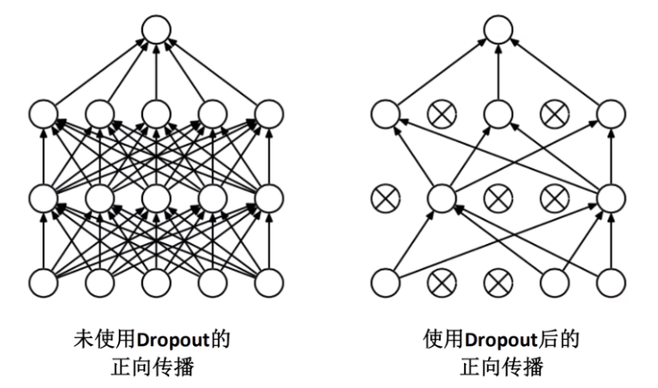
Dropout层
-
卷积池化后特征矩阵大小
-
view、unsqueeze、flatten函数
2.1网络亮点——GPU,ReLU,Dropout
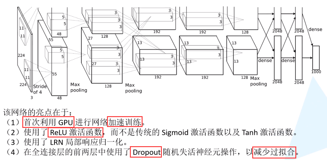
使用Dropout的方式在网络正向传播过程中随机失活一部分神经元,以减少过拟合
2.2 Conv1层
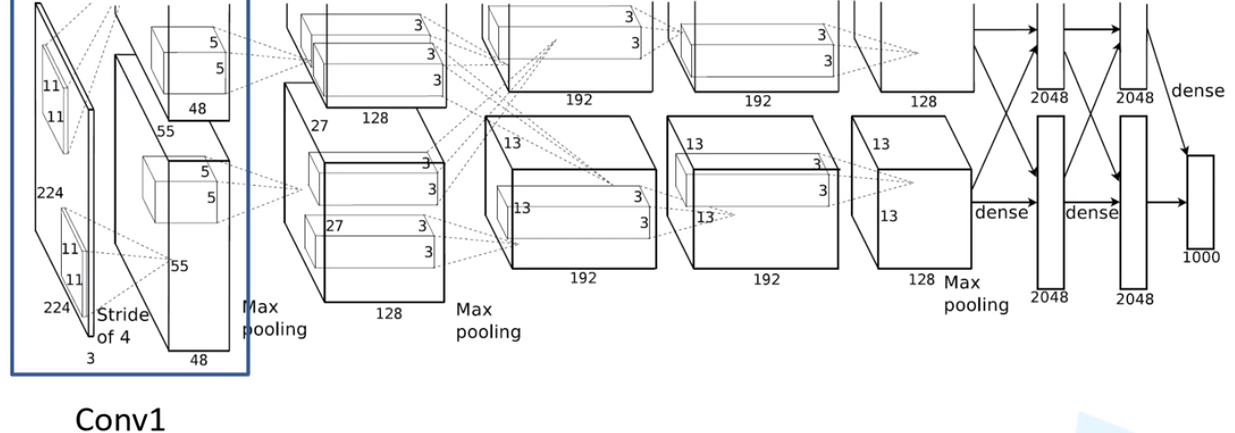
注意:原作者实验时用了两块GPU并行计算,上下两组图的结构是一样的。
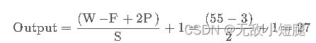
经 Conv1 卷积后的输出层尺寸为:
- 输入:input_size = [224, 224, 3]
- 输出:output_size = [55, 55, 96]
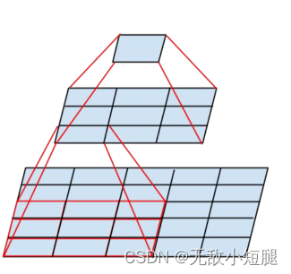
2.3 Maxpool1
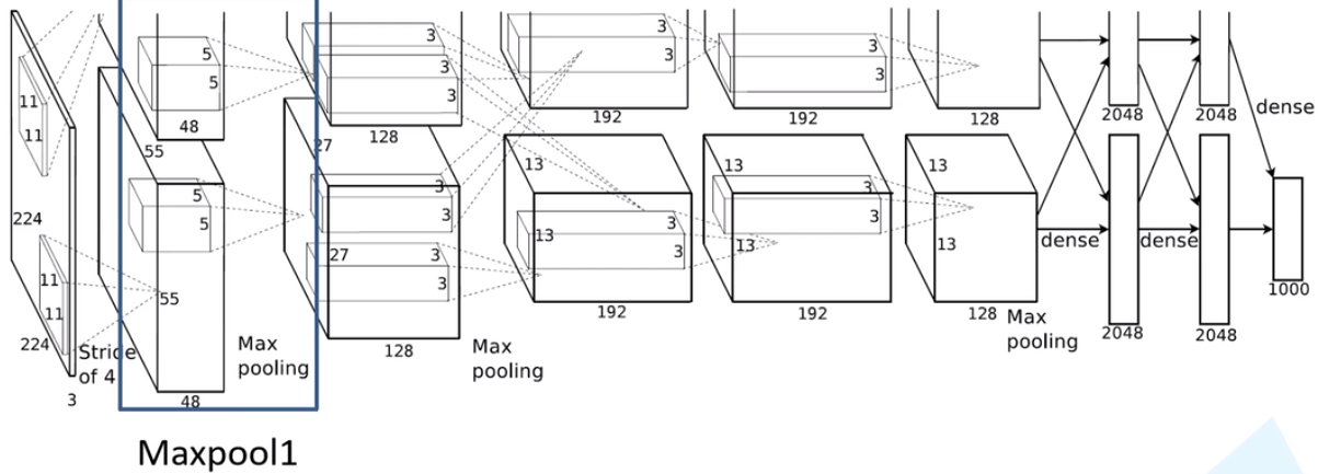
经 Maxpool1 后的输出层尺寸为:
- F与S均为2
- 输入:input_size = [55, 55, 96]
- 输出:output_size = [27, 27, 96]
分析可以发现,除 Conv1 外,AlexNet 的其余卷积层都是在改变特征矩阵的深度,而池化层则只改变(减小)其尺寸。
2.4 model.py
卷积池化层提取图像特征,全连接层进行图像分类,代码中写成两个模块,方便调用
- 模型:卷积、激活、池化、Dropout、线性
- 网络参数初始化:init_weights函数
- torch.flatten()展平
import torch.nn as nn
import torch

class AlexNet(nn.Module):
    def __init__(self, num_classes=1000, init_weights=False):
        super(AlexNet, self).__init__()
        # 用nn.Sequential()将网络打包成一个模块,精简代码
        self.features = nn.Sequential(   # 卷积层提取图像特征
            nn.Conv2d(3, 48, kernel_size=11, stride=4, padding=2),  # input[3, 224, 224]  output[48, 55, 55]
            nn.ReLU(inplace=True), 									# 直接修改覆盖原值,节省运算内存
            nn.MaxPool2d(kernel_size=3, stride=2),                  # output[48, 27, 27]
            nn.Conv2d(48, 128, kernel_size=5, padding=2),           # output[128, 27, 27]
            nn.ReLU(inplace=True),
            nn.MaxPool2d(kernel_size=3, stride=2),                  # output[128, 13, 13]
            nn.Conv2d(128, 192, kernel_size=3, padding=1),          # output[192, 13, 13]
            nn.ReLU(inplace=True),
            nn.Conv2d(192, 192, kernel_size=3, padding=1),          # output[192, 13, 13]
            nn.ReLU(inplace=True),
            nn.Conv2d(192, 128, kernel_size=3, padding=1),          # output[128, 13, 13]
            nn.ReLU(inplace=True),
            nn.MaxPool2d(kernel_size=3, stride=2),                  # output[128, 6, 6]
        )
        self.classifier = nn.Sequential(   # 全连接层对图像分类
            nn.Dropout(p=0.5),			   # Dropout 随机失活神经元,默认比例为0.5
            nn.Linear(128 * 6 * 6, 2048),
            nn.ReLU(inplace=True),
            nn.Dropout(p=0.5),
            nn.Linear(2048, 2048),
            nn.ReLU(inplace=True),
            nn.Linear(2048, num_classes),
        )
        if init_weights:
            self._initialize_weights()

	# 前向传播过程
    def forward(self, x):
        x = self.features(x)
        x = torch.flatten(x, start_dim=1)	# 展平后再传入全连接层
        x = self.classifier(x)
        return x

	# 网络权重初始化,实际上 pytorch 在构建网络时会自动初始化权重
    def _initialize_weights(self):
        for m in self.modules():
            if isinstance(m, nn.Conv2d):                            # 若是卷积层
                nn.init.kaiming_normal_(m.weight, mode='fan_out',   # 用(何)kaiming_normal_法初始化权重
                                        nonlinearity='relu')
                if m.bias is not None:
                    nn.init.constant_(m.bias, 0)                    # 初始化偏重为0
            elif isinstance(m, nn.Linear):            # 若是全连接层
                nn.init.normal_(m.weight, 0, 0.01)    # 正态分布初始化
                nn.init.constant_(m.bias, 0)          # 初始化偏重为0
3.模型训练、模型测试
注意:
-
借助GPU训练,to(device)添加位置
-
net.train(),net.eval()
-
torch.squeeze()、torch.unsqueeze()、torch.softmax()、torch.max()、torch.argmax()
训练过程中需要注意,以下两句语句尽量加,当有标准化和dropout层时候必须加
-
net.train():训练过程中开启 Dropout
-
net.eval(): 验证过程关闭 Dropout
3.1train.py
net = AlexNet(num_classes=5, init_weights=True)  	  # 实例化网络(输出类型为5,初始化权重)
net.to(device)									 	  # 分配网络到指定的设备(GPU/CPU)训练
loss_function = nn.CrossEntropyLoss()			 	  # 交叉熵损失
optimizer = optim.Adam(net.parameters(), lr=0.0002)	  # 优化器(训练参数,学习率)

save_path = './AlexNet.pth'
best_acc = 0.0

for epoch in range(10):
    ########################################## train ###############################################
    net.train()     					# 训练过程中开启 Dropout
    running_loss = 0.0					# 每个 epoch 都会对 running_loss  清零
    time_start = time.perf_counter()	# 对训练一个 epoch 计时

    for step, data in enumerate(train_loader, start=0):  # 遍历训练集,step从0开始计算
        images, labels = data   # 获取训练集的图像和标签
        optimizer.zero_grad()	# 清除历史梯度

        outputs = net(images.to(device))				 # 正向传播
        loss = loss_function(outputs, labels.to(device)) # 计算损失
        loss.backward()								     # 反向传播
        optimizer.step()								 # 优化器更新参数
        running_loss += loss.item()

        # 打印训练进度(使训练过程可视化)
        rate = (step + 1) / len(train_loader)           # 当前进度 = 当前step / 训练一轮epoch所需总step
        a = "*" * int(rate * 50)
        b = "." * int((1 - rate) * 50)
        print("\rtrain loss: {:^3.0f}%[{}->{}]{:.3f}".format(int(rate * 100), a, b, loss), end="")
    print()
    print('%f s' % (time.perf_counter()-time_start))

    ########################################### validate ###########################################
    net.eval()    # 验证过程中关闭 Dropout
    acc = 0.0
    with torch.no_grad():
        for val_data in validate_loader:
            val_images, val_labels = val_data
            outputs = net(val_images.to(device))
            predict_y = torch.max(outputs, dim=1)[1]  # 以output中值最大位置对应的索引(标签)作为预测输出
            acc += (predict_y == val_labels.to(device)).sum().item()
        val_accurate = acc / val_num

        # 保存准确率最高的那次网络参数
        if val_accurate > best_acc:
            best_acc = val_accurate
            torch.save(net.state_dict(), save_path)

        print('[epoch %d] train_loss: %.3f  test_accuracy: %.3f \n' %
              (epoch + 1, running_loss / step, val_accurate))

print('Finished Training')
3.2predict.py
import torch
from model import AlexNet
from PIL import Image
from torchvision import transforms
import matplotlib.pyplot as plt
import json

# 预处理
data_transform = transforms.Compose(
    [transforms.Resize((224, 224)),
     transforms.ToTensor(),
     transforms.Normalize((0.5, 0.5, 0.5), (0.5, 0.5, 0.5))])

# load image
img = Image.open("蒲公英.jpg")
plt.imshow(img)
# [N, C, H, W]
img = data_transform(img)
#增加第0个维度,即增加B
img = torch.unsqueeze(img, dim=0)

# read class_indict
try:
    json_file = open('./class_indices.json', 'r')
    class_indict = json.load(json_file)
except Exception as e:
    print(e)
    exit(-1)

# 创建一个模型,权重随机
model = AlexNet(num_classes=5)

# 加载已有模型
model_weight_path = "./AlexNet.pth"
model.load_state_dict(torch.load(model_weight_path))

# 关闭 Dropout
model.eval()
with torch.no_grad():
    # predict class
    output = torch.squeeze(model(img))     # 将输出压缩,即压缩掉 batch 这个维度
    predict = torch.softmax(output, dim=0)
    predict_cla = torch.argmax(predict).numpy()
print(class_indict[str(predict_cla)], predict[predict_cla].item())
plt.show()
四、VGG详解,感受野以及网络搭建
1.准备、划分、预处理、加载数据集:参照AlexNet
2.VGG模型详解
注意:特征提取层由外界参数传入
2.1多次小卷积核 代替 一次大卷积核
对于5*5矩阵,两次3*3卷积与一次5*5卷积效果相同,前者参数个数为2*3*3,后者参数为5*5
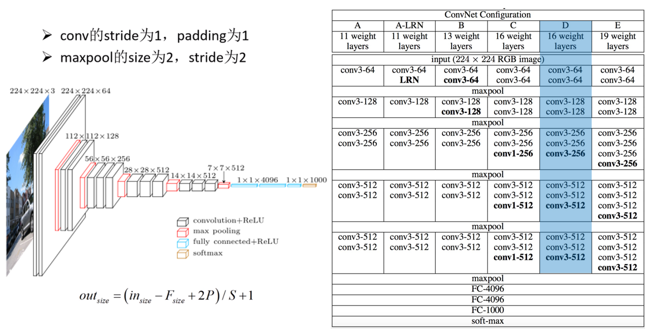
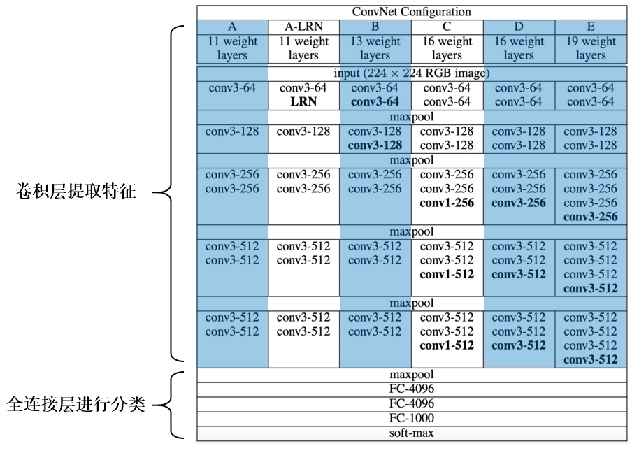
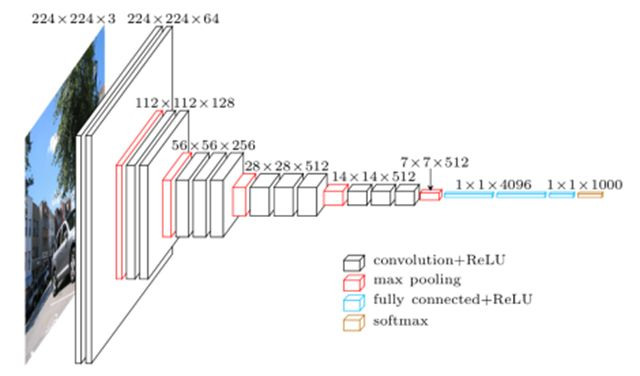
2.2网络结构图
2.3 model.py
跟上一篇中AlexNet网络模型的定义一样,VGG网络也是分为 卷积层提取特征 和 全连接层进行分类 这两个模块
import torch.nn as nn
import torch
class VGG(nn.Module):
def __init__(self, features, num_classes=1000, init_weights=False):
super(VGG, self).__init__()
self.features = features # 卷积层提取特征
self.classifier = nn.Sequential( # 全连接层进行分类
nn.Dropout(p=0.5),
nn.Linear(512*7*7, 2048),
nn.ReLU(True),
nn.Dropout(p=0.5),
nn.Linear(2048, 2048),
nn.ReLU(True),
nn.Linear(2048, num_classes)
)
if init_weights:
self._initialize_weights()
def forward(self, x):
# N x 3 x 224 x 224
x = self.features(x)
# N x 512 x 7 x 7
x = torch.flatten(x, start_dim=1)
# N x 512*7*7
x = self.classifier(x)
return x
def _initialize_weights(self):
for m in self.modules():
if isinstance(m, nn.Conv2d):
# nn.init.kaiming_normal_(m.weight, mode='fan_out', nonlinearity='relu')
nn.init.xavier_uniform_(m.weight)
if m.bias is not None:
nn.init.constant_(m.bias, 0)
elif isinstance(m, nn.Linear):
nn.init.xavier_uniform_(m.weight)
# nn.init.normal_(m.weight, 0, 0.01)
nn.init.constant_(m.bias, 0)
# vgg网络模型配置列表,数字表示卷积核个数,'M'表示最大池化层
cfgs = {
'vgg11': [64, 'M', 128, 'M', 256, 256, 'M', 512, 512, 'M', 512, 512, 'M'], # 模型A
'vgg13': [64, 64, 'M', 128, 128, 'M', 256, 256, 'M', 512, 512, 'M', 512, 512, 'M'], # 模型B
'vgg16': [64, 64, 'M', 128, 128, 'M', 256, 256, 256, 'M', 512, 512, 512, 'M', 512, 512, 512, 'M'], # 模型D
'vgg19': [64, 64, 'M', 128, 128, 'M', 256, 256, 256, 256, 'M', 512, 512, 512, 512, 'M', 512, 512, 512, 512, 'M'], # 模型E
}
# 卷积层提取特征
def make_features(cfg: list): # 传入的是具体某个模型的参数列表
layers = []
in_channels = 3 # 输入的原始图像(rgb三通道)
for v in cfg:
# 最大池化层
if v == "M":
layers += [nn.MaxPool2d(kernel_size=2, stride=2)]
# 卷积层
else:
conv2d = nn.Conv2d(in_channels, v, kernel_size=3, padding=1)
layers += [conv2d, nn.ReLU(True)]
in_channels = v
return nn.Sequential(*layers) # 单星号(*)将参数以元组(tuple)的形式导入
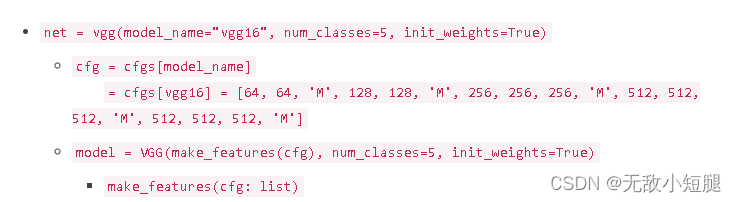
def vgg(model_name="vgg16", **kwargs): # 双星号(**)将参数以字典的形式导入
try:
cfg = cfgs[model_name]
except:
print("Warning: model number {} not in cfgs dict!".format(model_name))
exit(-1)
model = VGG(make_features(cfg), **kwargs)
return model
3.模型训练、模型测试
3.1train.py
训练脚本与AlexNet基本一致,需要注意的是实例化网络的过程:
model_name = "vgg16"
net = vgg(model_name=model_name, num_classes=5, init_weights=True)
函数调用关系:
3.2predict.py
预测脚本也跟AlexNet一致
五、GoogLeNet网络详解
原论文地址:Going deeper with convolutions
GoogLeNet 的创新点:
- 引入了 Inception 结构(融合不同尺度的特征信息)
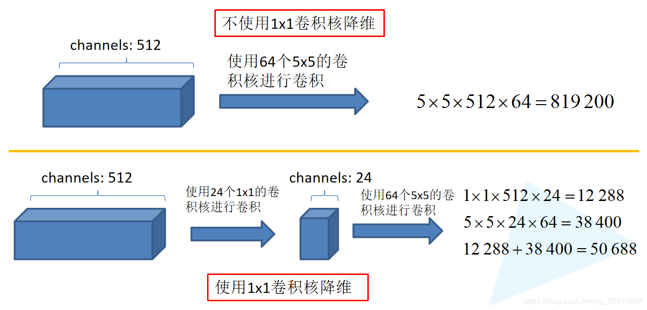
- 使用1x1的卷积核进行降维以及映射处理 (虽然VGG网络中也有,但该论文介绍的更详细)
- 添加两个辅助分类器帮助训练
- 丢弃全连接层,使用平均池化层(大大减少模型参数,除去两个辅助分类器,网络大小只有vgg的1/20)
1.准备、划分、预处理、加载数据集:参照AlexNet
2.GoogLeNet详解
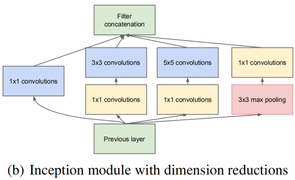
2.1Inception结构
- 传统的CNN结构如AlexNet、VggNet(下图)都是串联的结构,即将一系列的卷积层和池化层进行串联得到的结构。
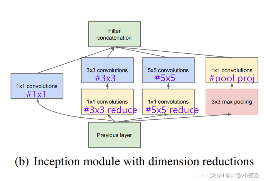
- GoogLeNet 提出了一种并联结构,下图是论文中提出的inception结构,将特征矩阵同时输入到多个分支进行处理,并将输出的特征矩阵按深度进行拼接,得到最终输出。其中1*1卷积层作用是降维。
-
对于Inception模块,所需要使用到参数#1x1, #3x3reduce, #3x3, #5x5reduce, #5x5, poolproj,这6个参数,分别对应着所使用的卷积核个数。
-
#1x1对应着分支1上1x1的卷积核个数
-
#3x3reduce对应着分支2上1x1的卷积核个数
-
#3x3对应着分支2上3x3的卷积核个数
-
#5x5reduce对应着分支3上1x1的卷积核个数
-
#5x5对应着分支3上5x5的卷积核个数
-
poolproj对应着分支4上1x1的卷积核个数。
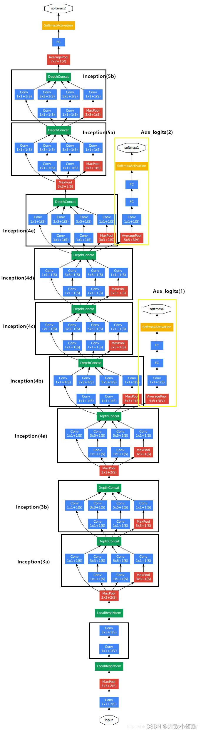
2.2辅助分类器(Auxiliary Classifier)
- AlexNet 和 VGG 都只有1个输出层,GoogLeNet 有3个输出层,其中的两个是辅助分类层。
- 辅助分类器的两个分支有什么用呢?
- 作用一:可以把他看做inception网络中的一个小细节,它确保了即便是隐藏单元和中间层也参与了特征计算,他们也能预测图片的类别,他在inception网络中起到一种调整的效果,并且能防止网络发生过拟合。
- 作用二:给定深度相对较大的网络,有效传播梯度反向通过所有层的能力是一个问题。通过将辅助分类器添加到这些中间层,可以期望较低阶段分类器的判别力。在训练期间,它们的损失以折扣权重(辅助分类器损失的权重是0.3)加到网络的整个损失上。
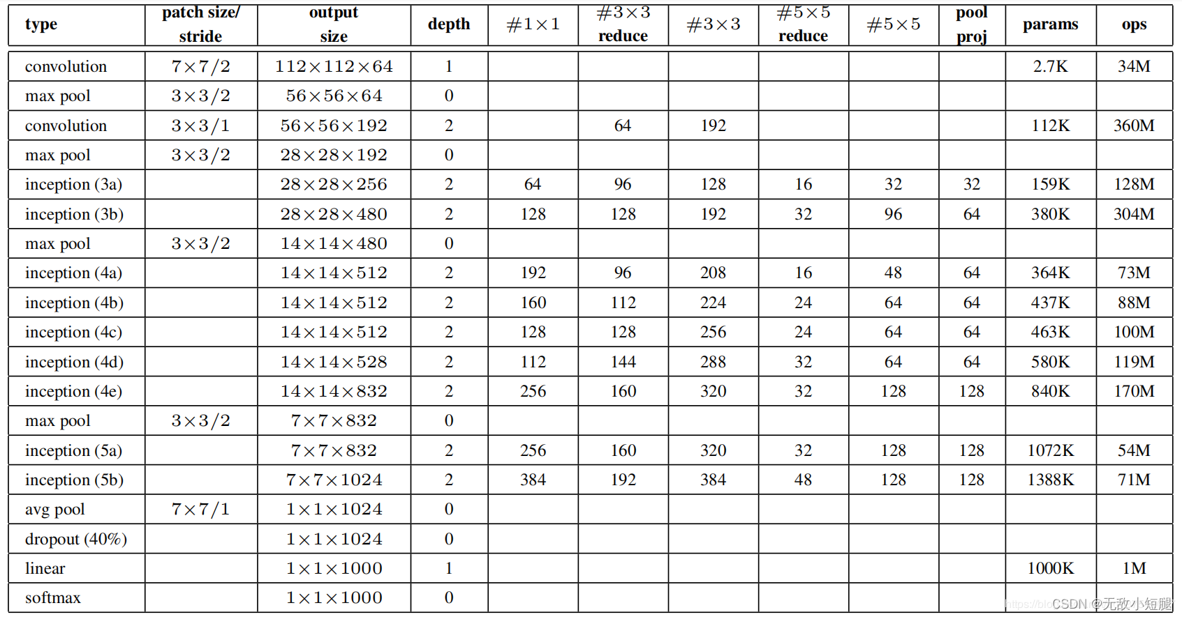
2.3 GoogLeNet网络参数
2.4model.py
相比于 AlexNet 和 VggNet 只有卷积层和全连接层这两种结构,GoogLeNet多了 inception 和 辅助分类器(Auxiliary Classifier),而 inception 和 辅助分类器 也是由多个卷积层和全连接层组合的,因此在定义模型时可以将 卷积、inception 、辅助分类器定义成不同的类,调用时更加方便。
import torch.nn as nn
import torch
import torch.nn.functional as F

class GoogLeNet(nn.Module):
	# 传入的参数中aux_logits=True表示训练过程用到辅助分类器,aux_logits=False表示验证过程不用辅助分类器
    def __init__(self, num_classes=1000, aux_logits=True, init_weights=False):
        super(GoogLeNet, self).__init__()
        self.aux_logits = aux_logits

        #BasicConv2d类中包括卷积和relu两个操作
        self.conv1 = BasicConv2d(3, 64, kernel_size=7, stride=2, padding=3)
        self.maxpool1 = nn.MaxPool2d(3, stride=2, ceil_mode=True)

        self.conv2 = BasicConv2d(64, 64, kernel_size=1)
        self.conv3 = BasicConv2d(64, 192, kernel_size=3, padding=1)
        self.maxpool2 = nn.MaxPool2d(3, stride=2, ceil_mode=True)

        self.inception3a = Inception(192, 64, 96, 128, 16, 32, 32)
        self.inception3b = Inception(256, 128, 128, 192, 32, 96, 64)
        self.maxpool3 = nn.MaxPool2d(3, stride=2, ceil_mode=True)

        self.inception4a = Inception(480, 192, 96, 208, 16, 48, 64)
        self.inception4b = Inception(512, 160, 112, 224, 24, 64, 64)
        self.inception4c = Inception(512, 128, 128, 256, 24, 64, 64)
        self.inception4d = Inception(512, 112, 144, 288, 32, 64, 64)
        self.inception4e = Inception(528, 256, 160, 320, 32, 128, 128)
        self.maxpool4 = nn.MaxPool2d(3, stride=2, ceil_mode=True)

        self.inception5a = Inception(832, 256, 160, 320, 32, 128, 128)
        self.inception5b = Inception(832, 384, 192, 384, 48, 128, 128)

        if self.aux_logits:
            self.aux1 = InceptionAux(512, num_classes)
            self.aux2 = InceptionAux(528, num_classes)

        self.avgpool = nn.AdaptiveAvgPool2d((1, 1))
        self.dropout = nn.Dropout(0.4)
        self.fc = nn.Linear(1024, num_classes)
        if init_weights:
            self._initialize_weights()

    def forward(self, x):
        # N x 3 x 224 x 224
        x = self.conv1(x)
        # N x 64 x 112 x 112
        x = self.maxpool1(x)
        # N x 64 x 56 x 56
        x = self.conv2(x)
        # N x 64 x 56 x 56
        x = self.conv3(x)
        # N x 192 x 56 x 56
        x = self.maxpool2(x)

        # N x 192 x 28 x 28
        x = self.inception3a(x)
        # N x 256 x 28 x 28
        x = self.inception3b(x)
        # N x 480 x 28 x 28
        x = self.maxpool3(x)
        # N x 480 x 14 x 14
        x = self.inception4a(x)
        # N x 512 x 14 x 14
        if self.training and self.aux_logits:    # eval model lose this layer
            aux1 = self.aux1(x)

        x = self.inception4b(x)
        # N x 512 x 14 x 14
        x = self.inception4c(x)
        # N x 512 x 14 x 14
        x = self.inception4d(x)
        # N x 528 x 14 x 14
        if self.training and self.aux_logits:    # eval model lose this layer
            aux2 = self.aux2(x)

        x = self.inception4e(x)
        # N x 832 x 14 x 14
        x = self.maxpool4(x)
        # N x 832 x 7 x 7
        x = self.inception5a(x)
        # N x 832 x 7 x 7
        x = self.inception5b(x)
        # N x 1024 x 7 x 7

        x = self.avgpool(x)
        # N x 1024 x 1 x 1
        x = torch.flatten(x, 1)
        # N x 1024
        x = self.dropout(x)
        x = self.fc(x)
        # N x 1000 (num_classes)
        if self.training and self.aux_logits:   # eval model lose this layer
            return x, aux2, aux1
        return x

    def _initialize_weights(self):
        for m in self.modules():
            if isinstance(m, nn.Conv2d):
                nn.init.kaiming_normal_(m.weight, mode='fan_out', nonlinearity='relu')
                if m.bias is not None:
                    nn.init.constant_(m.bias, 0)
            elif isinstance(m, nn.Linear):
                nn.init.normal_(m.weight, 0, 0.01)
                nn.init.constant_(m.bias, 0)

# Inception结构
class Inception(nn.Module):
    def __init__(self, in_channels, ch1x1, ch3x3red, ch3x3, ch5x5red, ch5x5, pool_proj):
        super(Inception, self).__init__()

        self.branch1 = BasicConv2d(in_channels, ch1x1, kernel_size=1)

        self.branch2 = nn.Sequential(
            BasicConv2d(in_channels, ch3x3red, kernel_size=1),
            BasicConv2d(ch3x3red, ch3x3, kernel_size=3, padding=1)   # 保证输出大小等于输入大小
        )

        self.branch3 = nn.Sequential(
            BasicConv2d(in_channels, ch5x5red, kernel_size=1),
            BasicConv2d(ch5x5red, ch5x5, kernel_size=5, padding=2)   # 保证输出大小等于输入大小
        )

        self.branch4 = nn.Sequential(
            nn.MaxPool2d(kernel_size=3, stride=1, padding=1),
            BasicConv2d(in_channels, pool_proj, kernel_size=1)
        )

    def forward(self, x):
        branch1 = self.branch1(x)
        branch2 = self.branch2(x)
        branch3 = self.branch3(x)
        branch4 = self.branch4(x)

        outputs = [branch1, branch2, branch3, branch4]
        return torch.cat(outputs, 1) # 按 channel 对四个分支拼接

# 辅助分类器
class InceptionAux(nn.Module):
    def __init__(self, in_channels, num_classes):
        super(InceptionAux, self).__init__()
        self.averagePool = nn.AvgPool2d(kernel_size=5, stride=3)
        self.conv = BasicConv2d(in_channels, 128, kernel_size=1)  # output[batch, 128, 4, 4]

        self.fc1 = nn.Linear(2048, 1024)
        self.fc2 = nn.Linear(1024, num_classes)

    def forward(self, x):
        # aux1: N x 512 x 14 x 14, aux2: N x 528 x 14 x 14
        x = self.averagePool(x)
        # aux1: N x 512 x 4 x 4, aux2: N x 528 x 4 x 4
        x = self.conv(x)
        # N x 128 x 4 x 4
        x = torch.flatten(x, 1)
        x = F.dropout(x, 0.5, training=self.training)
        # N x 2048
        x = F.relu(self.fc1(x), inplace=True)
        x = F.dropout(x, 0.5, training=self.training)
        # N x 1024
        x = self.fc2(x)
        # N x num_classes
        return x

# 基础卷积层(卷积+ReLU)
class BasicConv2d(nn.Module):
    def __init__(self, in_channels, out_channels, **kwargs):
        super(BasicConv2d, self).__init__()
        self.conv = nn.Conv2d(in_channels, out_channels, **kwargs)
        self.relu = nn.ReLU(inplace=True)

    def forward(self, x):
        x = self.conv(x)
        x = self.relu(x)
        return x
3.模型训练、模型测试
3.1 train.py
net = GoogLeNet(num_classes=5, aux_logits=True, init_weights=True)
- GoogLeNet的网络输出 loss 有三个部分,分别是主干输出loss、两个辅助分类器输出loss(权重0.3)
logits, aux_logits2, aux_logits1 = net(images.to(device))
loss0 = loss_function(logits, labels.to(device))
loss1 = loss_function(aux_logits1, labels.to(device))
loss2 = loss_function(aux_logits2, labels.to(device))
loss = loss0 + loss1 * 0.3 + loss2 * 0.3
3.2 predict.py
预测部分跟AlexNet和VGG类似,需要注意在实例化模型时不需要 辅助分类器
# create model
model = GoogLeNet(num_classes=5, aux_logits=False)

# load model weights
model_weight_path = "./googleNet.pth"

missing_keys, unexpected_keys = model.load_state_dict(torch.load(model_weight_path), strict=False)
六、ResNet网络详解与迁移学习
1.准备、划分、预处理、加载数据集:参照AlexNet
2.ResNet详解
2.1 创新点
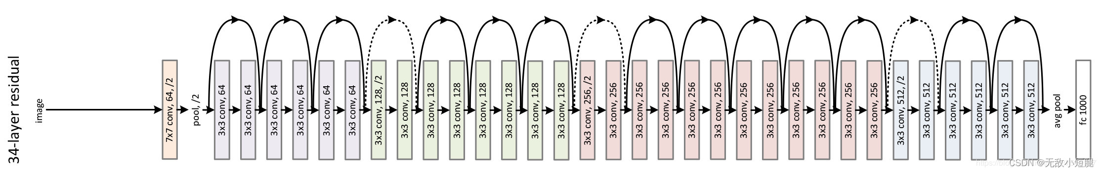
- 提出 Residual 结构(残差结构),并搭建超深的网络结构(可突破1000层)
- 使用 Batch Normalization 加速训练(丢弃dropout)
下图·是·34层模型简图:
2.2 什么是残差?
为了解决深层网络中的退化问题,可以人为地让神经网络某些层跳过下一层神经元的连接,隔层相连,弱化每层之间的强联系。这种神经网络被称为 残差网络 (ResNets)。
残差网络由许多隔层相连的神经元子模块组成,我们称之为 残差块 Residual block。单个残差块的结构如下图所示:
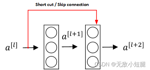
上图中红色部分称为 short cut 或者 skip connection(也称 捷径分支),直接建立![a^{[l]}](https://latex.csdn.net/eq?a%5E%7B%5Bl%5D%7D) 与
与![a^{[l+2]}](https://latex.csdn.net/eq?a%5E%7B%5Bl+2%5D%7D)
之间的隔层联系。其前向传播的计算步骤为:
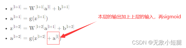
直接隔层与下一层的线性输出相连,与![z^{[l+2]}](https://latex.csdn.net/eq?z%5E%7B%5Bl+2%5D%7D) 共同通过激活函数(ReLU)输出 。
共同通过激活函数(ReLU)输出 。
由多个 残差块 组成的神经网络就是 残差网络 。其结构如下图所示:
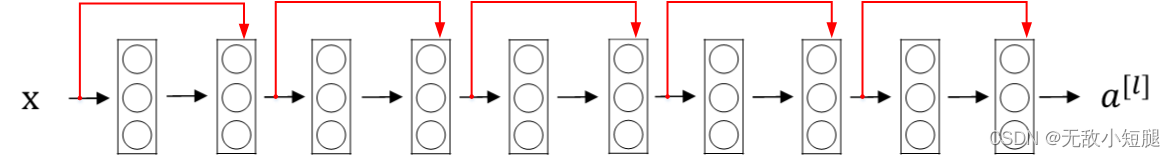
关键:这一层的输入(经过激活函数)与下一层的输出(未经过激活函数)相加,后再使用激活函数
2.3 为什么使用残差?
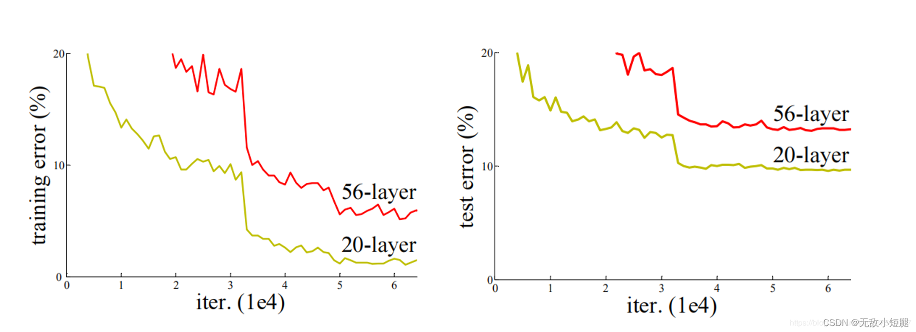
在ResNet网络提出之前,传统的卷积神经网络都是通过将一系列卷积层与池化层进行堆叠得到的。一般我们会觉得网络越深,特征信息越丰富,模型效果应该越好。但是实验证明,当网络堆叠到一定深度时,会出现两个问题:
关于梯度消失和梯度爆炸,其实看名字理解最好:
若每一层的误差梯度小于1,反向传播时,网络越深,梯度越趋近于0
反之,若每一层的误差梯度大于1,反向传播时,网路越深,梯度越来越大
-
退化问题(degradation problem):在解决了梯度消失、爆炸问题后,仍然存在深层网络的效果可能比浅层网络差的现象
总结就是,当网络堆叠到一定深度时,反而会出现深层网络比浅层网络效果差的情况。
如下图所示,20层网络 反而比 56层网络 的误差更小:
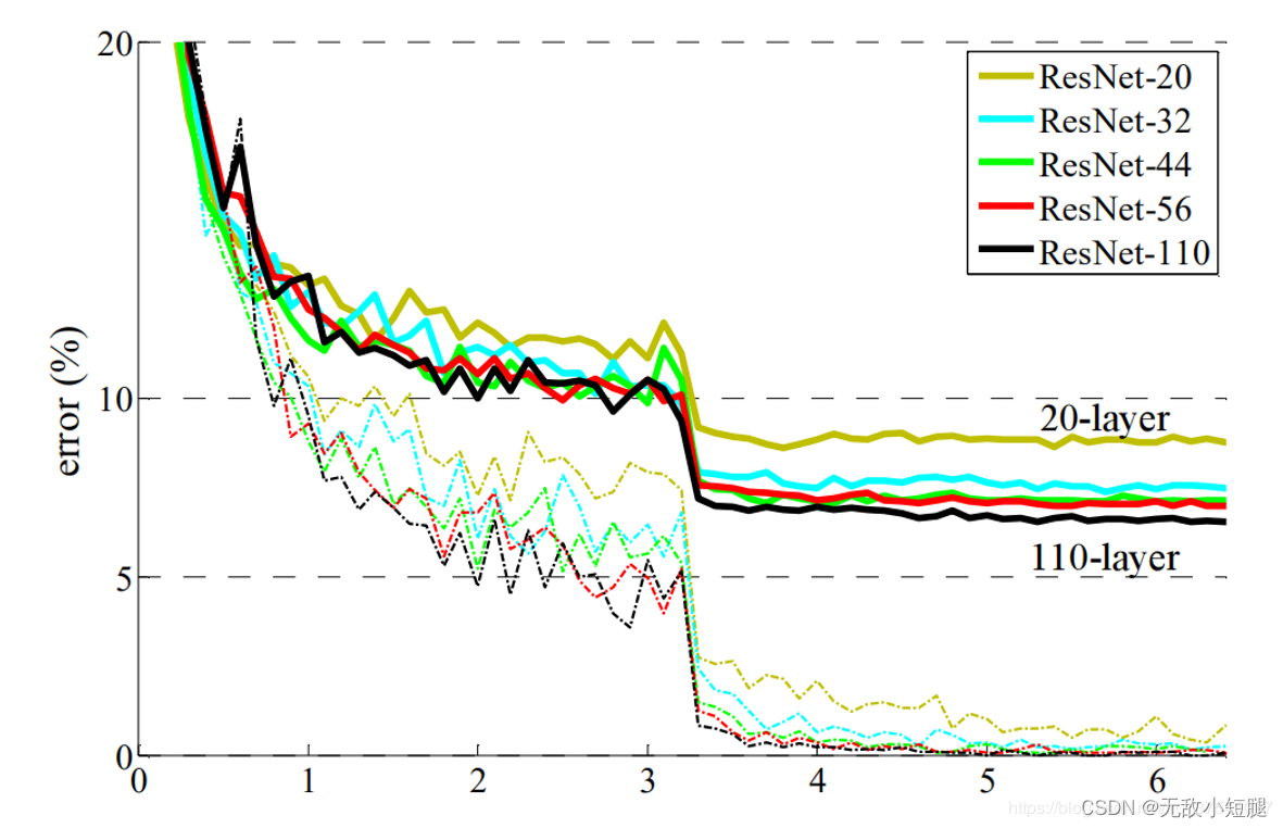
- 对于梯度消失或梯度爆炸问题,ResNet论文提出通过数据的预处理以及在网络中使用 BN(Batch Normalization)层来解决。
- 对于退化问题,ResNet论文提出了 residual结构(残差结构)来减轻退化问题,下图是使用residual结构的卷积网络,可以看到随着网络的不断加深,效果并没有变差,而是变的更好了。(虚线是train error,实线是test error)
2.4 ResNet中的残差结构
- 实际应用中,残差结构的 short cut 不一定是隔一层连接,也可以中间隔多层,ResNet所提出的残差网络中就是隔多层。
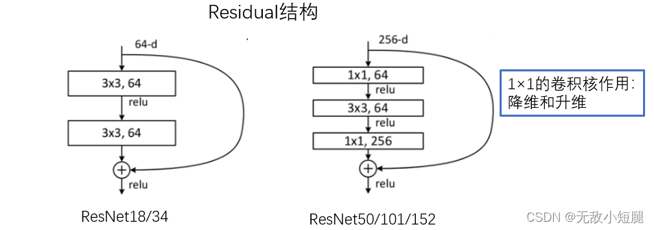
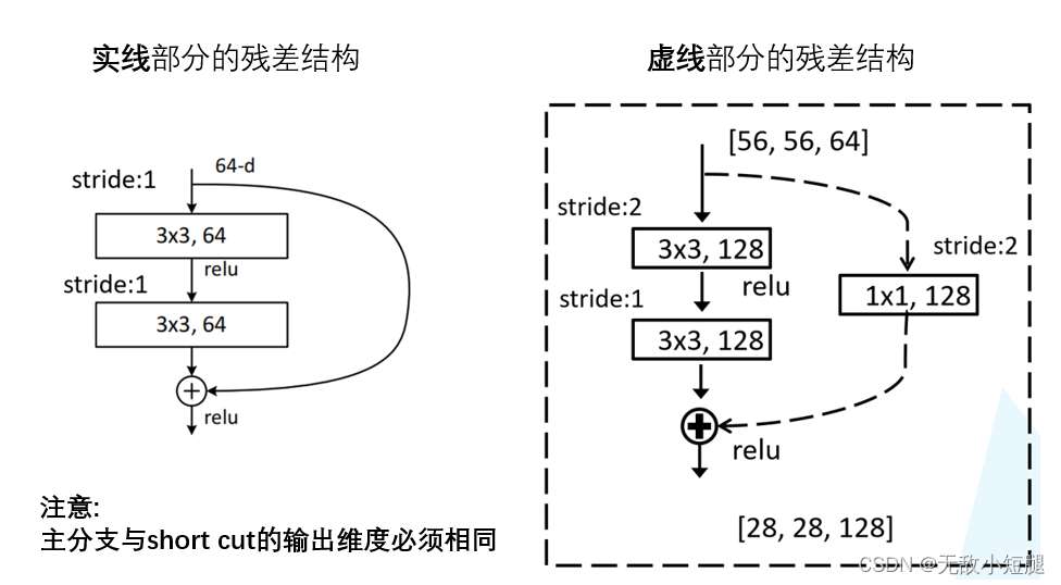
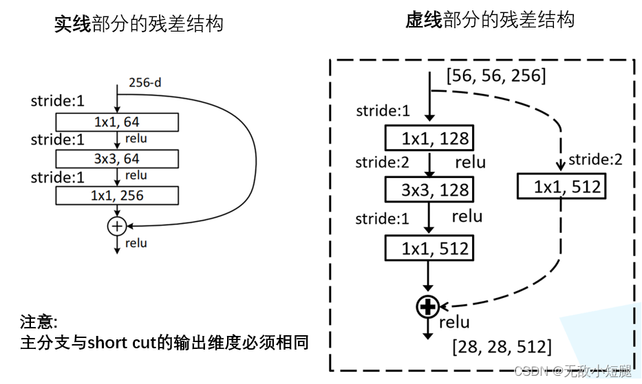
- 跟VggNet类似,ResNet也有多个不同层的版本,而残差结构也有两种对应浅层和深层网络:
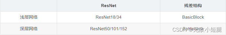
- 下图中左侧残差结构称为 BasicBlock,右侧残差结构称为 Bottleneck
2.5 降维时的short cut
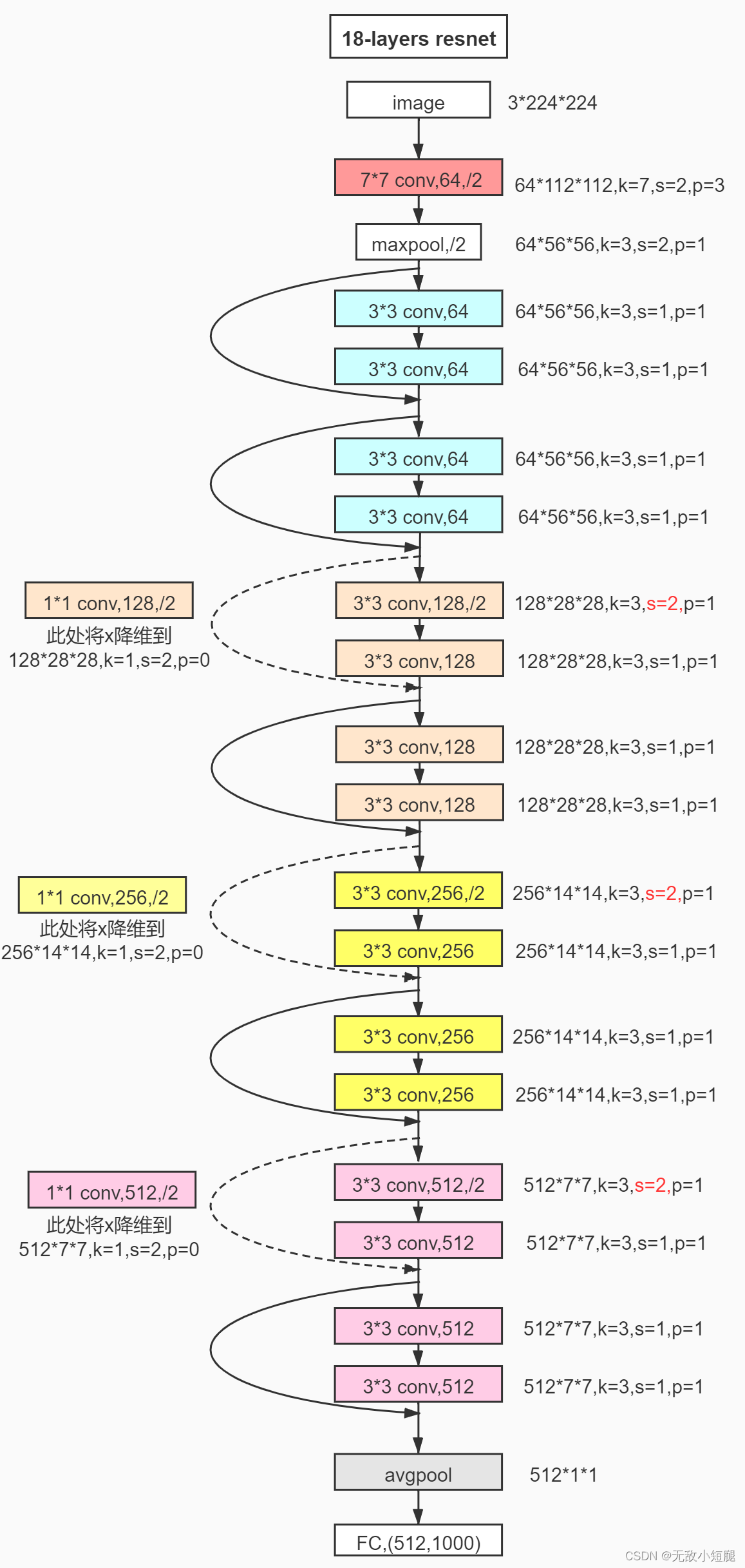
观察下图的 ResNet18层网络,可以发现有些残差块的 short cut 是实线的,而有些则是虚线的。
这些虚线的 short cut 上通过1×1的卷积核进行了维度处理(特征矩阵在长宽方向降采样,深度方向调整成下一层残差结构所需要的channel)。
2.6 model.py
import torch.nn as nn
import torch


# ResNet18/34的残差结构,用的是2个3x3的卷积
class BasicBlock(nn.Module):
    expansion = 1  # 残差结构中,主分支的卷积核个数是否发生变化,不变则为1

    def __init__(self, in_channel, out_channel, stride=1, downsample=None):  # downsample对应虚线残差结构
        super(BasicBlock, self).__init__()
        self.conv1 = nn.Conv2d(in_channels=in_channel, out_channels=out_channel,
                               kernel_size=3, stride=stride, padding=1, bias=False)
        self.bn1 = nn.BatchNorm2d(out_channel)
        self.relu = nn.ReLU()
        self.conv2 = nn.Conv2d(in_channels=out_channel, out_channels=out_channel,
                               kernel_size=3, stride=1, padding=1, bias=False)
        self.bn2 = nn.BatchNorm2d(out_channel)
        self.downsample = downsample

    def forward(self, x):
        identity = x
        if self.downsample is not None:  # 虚线残差结构,需要下采样
            identity = self.downsample(x)  # 捷径分支 short cut

        out = self.conv1(x)
        out = self.bn1(out)
        out = self.relu(out)

        out = self.conv2(out)
        out = self.bn2(out)

        out += identity
        out = self.relu(out)

        return out

# ResNet50/101/152的残差结构,用的是1x1+3x3+1x1的卷积
class Bottleneck(nn.Module):
    expansion = 4  # 残差结构中第三层卷积核个数是第一/二层卷积核个数的4倍

    def __init__(self, in_channel, out_channel, stride=1, downsample=None):
        super(Bottleneck, self).__init__()
        self.conv1 = nn.Conv2d(in_channels=in_channel, out_channels=out_channel,
                               kernel_size=1, stride=1, bias=False)  # squeeze channels
        self.bn1 = nn.BatchNorm2d(out_channel)
        # -----------------------------------------
        self.conv2 = nn.Conv2d(in_channels=out_channel, out_channels=out_channel,
                               kernel_size=3, stride=stride, bias=False, padding=1)
        self.bn2 = nn.BatchNorm2d(out_channel)
        # -----------------------------------------
        self.conv3 = nn.Conv2d(in_channels=out_channel, out_channels=out_channel * self.expansion,
                               kernel_size=1, stride=1, bias=False)  # unsqueeze channels
        self.bn3 = nn.BatchNorm2d(out_channel * self.expansion)
        self.relu = nn.ReLU(inplace=True)
        self.downsample = downsample

    def forward(self, x):
        identity = x
        if self.downsample is not None:
            identity = self.downsample(x)  # 捷径分支 short cut

        out = self.conv1(x)
        out = self.bn1(out)
        out = self.relu(out)

        out = self.conv2(out)
        out = self.bn2(out)
        out = self.relu(out)

        out = self.conv3(out)
        out = self.bn3(out)

        out += identity
        out = self.relu(out)

        return out


class ResNet(nn.Module):
    # block = BasicBlock or Bottleneck
    # block_num为残差结构中conv2_x~conv5_x中残差块个数,是一个列表
    def __init__(self, block, blocks_num, num_classes=1000, include_top=True):
        super(ResNet, self).__init__()
        self.include_top = include_top
        self.in_channel = 64

        self.conv1 = nn.Conv2d(3, self.in_channel, kernel_size=7, stride=2,
                               padding=3, bias=False)
        self.bn1 = nn.BatchNorm2d(self.in_channel)
        self.relu = nn.ReLU(inplace=True)
        self.maxpool = nn.MaxPool2d(kernel_size=3, stride=2, padding=1)
        self.layer1 = self._make_layer(block, 64, blocks_num[0])             # conv2_x
        self.layer2 = self._make_layer(block, 128, blocks_num[1], stride=2)  # conv3_x
        self.layer3 = self._make_layer(block, 256, blocks_num[2], stride=2)  # conv4_x
        self.layer4 = self._make_layer(block, 512, blocks_num[3], stride=2)  # conv5_x
        if self.include_top:
            self.avgpool = nn.AdaptiveAvgPool2d((1, 1))  # output size = (1, 1)
            self.fc = nn.Linear(512 * block.expansion, num_classes)

        for m in self.modules():
            if isinstance(m, nn.Conv2d):
                nn.init.kaiming_normal_(m.weight, mode='fan_out', nonlinearity='relu')

    # channel为残差结构中第一层卷积核个数
    def _make_layer(self, block, channel, block_num, stride=1):
        downsample = None

        # ResNet50/101/152的残差结构,block.expansion=4
        if stride != 1 or self.in_channel != channel * block.expansion:
            downsample = nn.Sequential(
                nn.Conv2d(self.in_channel, channel * block.expansion, kernel_size=1, stride=stride, bias=False),
                nn.BatchNorm2d(channel * block.expansion))

        layers = []
        layers.append(block(self.in_channel, channel, downsample=downsample, stride=stride))
        self.in_channel = channel * block.expansion

        for _ in range(1, block_num):
            layers.append(block(self.in_channel, channel))

        return nn.Sequential(*layers)

    def forward(self, x):
        x = self.conv1(x)
        x = self.bn1(x)
        x = self.relu(x)
        x = self.maxpool(x)

        x = self.layer1(x)
        x = self.layer2(x)
        x = self.layer3(x)
        x = self.layer4(x)

        if self.include_top:
            x = self.avgpool(x)
            x = torch.flatten(x, 1)
            x = self.fc(x)

        return x


def resnet34(num_classes=1000, include_top=True):
    return ResNet(BasicBlock, [3, 4, 6, 3], num_classes=num_classes, include_top=include_top)


def resnet101(num_classes=1000, include_top=True):
    return ResNet(Bottleneck, [3, 4, 23, 3], num_classes=num_classes, include_top=include_top)
3.迁移学习
3.1 简介
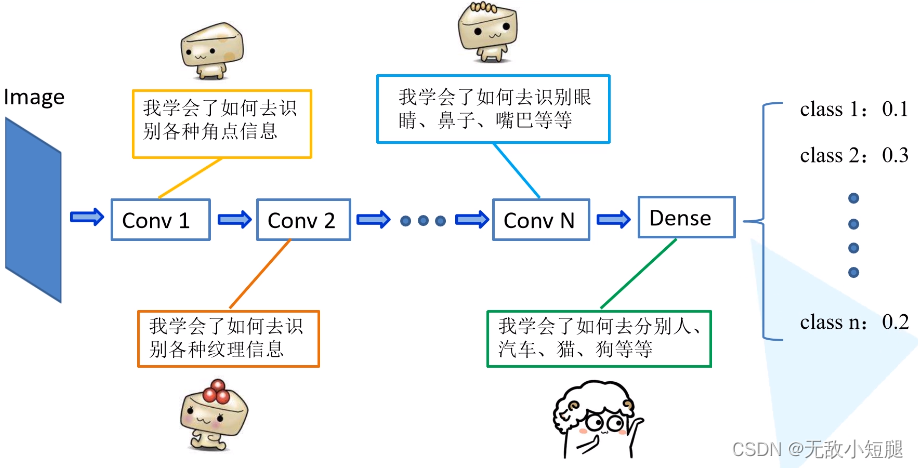
例如,一个训练好的图像分类网络能够被用于另一个图像相关的任务。再比如,一个网络在仿真环境学习的知识可以被迁移到真实环境的网络。迁移学习一个典型的例子就是载入训练好VGG网络,这个大规模分类网络能将图像分到1000个类别,然后把这个网络用于另一个任务,如医学图像分类。
为什么可以这么做呢?如下图所示,神经网络逐层提取图像的深层信息,这样,预训练网络就相当于一个特征提取器。
3.2 优势
-
能够快速的训练出一个理想的结果
-
当数据集较小时也能训练出理想的效果
注意:使用别人预训练好的模型参数时,要注意别人的预处理方式。
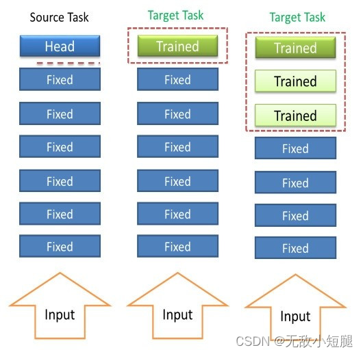
3.3 常见的学习方式
- 载入权重后训练所有参数
- 载入权重后只训练最后几层参数
- 载入权重后在原网络基础上再添加一层全连接层,仅训练最后一个全连接层
4.模型训练、模型测试
4.1 train.py
import torch
import torch.nn as nn
from torchvision import transforms, datasets
import json
import matplotlib.pyplot as plt
import os
import torch.optim as optim
from model import resnet34, resnet101
import torchvision.models.resnet


device = torch.device("cuda:0" if torch.cuda.is_available() else "cpu")
print(device)

data_transform = {
    "train": transforms.Compose([transforms.RandomResizedCrop(224),
                                 transforms.RandomHorizontalFlip(),
                                 transforms.ToTensor(),
                                 transforms.Normalize([0.485, 0.456, 0.406], [0.229, 0.224, 0.225])]),
    "val": transforms.Compose([transforms.Resize(256),
                               transforms.CenterCrop(224),
                               transforms.ToTensor(),
                               transforms.Normalize([0.485, 0.456, 0.406], [0.229, 0.224, 0.225])])}


data_root = os.path.abspath(os.path.join(os.getcwd(), "../.."))  # get data root path
image_path = data_root + "/data_set/flower_data/"  # flower data set path

train_dataset = datasets.ImageFolder(root=image_path+"train",
                                     transform=data_transform["train"])
train_num = len(train_dataset)

# {'daisy':0, 'dandelion':1, 'roses':2, 'sunflower':3, 'tulips':4}
flower_list = train_dataset.class_to_idx
cla_dict = dict((val, key) for key, val in flower_list.items())
# write dict into json file
json_str = json.dumps(cla_dict, indent=4)
with open('class_indices.json', 'w') as json_file:
    json_file.write(json_str)

batch_size = 16
train_loader = torch.utils.data.DataLoader(train_dataset,
                                           batch_size=batch_size, shuffle=True,
                                           num_workers=0)

validate_dataset = datasets.ImageFolder(root=image_path + "val",
                                        transform=data_transform["val"])
val_num = len(validate_dataset)
validate_loader = torch.utils.data.DataLoader(validate_dataset,
                                              batch_size=batch_size, shuffle=False,
                                              num_workers=0)

net = resnet34()
# load pretrain weights
model_weight_path = "./resnet34-pre.pth"
missing_keys, unexpected_keys = net.load_state_dict(torch.load(model_weight_path), strict=False)
# for param in net.parameters():
#     param.requires_grad = False
# change fc layer structure
inchannel = net.fc.in_features
net.fc = nn.Linear(inchannel, 5)
net.to(device)

loss_function = nn.CrossEntropyLoss()
optimizer = optim.Adam(net.parameters(), lr=0.0001)

best_acc = 0.0
save_path = './resNet34.pth'
for epoch in range(3):
    # train
    net.train()
    running_loss = 0.0
    for step, data in enumerate(train_loader, start=0):
        images, labels = data
        optimizer.zero_grad()
        logits = net(images.to(device))
        loss = loss_function(logits, labels.to(device))
        loss.backward()
        optimizer.step()

        # print statistics
        running_loss += loss.item()
        # print train process
        rate = (step+1)/len(train_loader)
        a = "*" * int(rate * 50)
        b = "." * int((1 - rate) * 50)
        print("\rtrain loss: {:^3.0f}%[{}->{}]{:.4f}".format(int(rate*100), a, b, loss), end="")
    print()

    # validate
    net.eval()
    acc = 0.0  # accumulate accurate number / epoch
    with torch.no_grad():
        for val_data in validate_loader:
            val_images, val_labels = val_data
            outputs = net(val_images.to(device))  # eval model only have last output layer
            # loss = loss_function(outputs, test_labels)
            predict_y = torch.max(outputs, dim=1)[1]
            acc += (predict_y == val_labels.to(device)).sum().item()
        val_accurate = acc / val_num
        if val_accurate > best_acc:
            best_acc = val_accurate
            torch.save(net.state_dict(), save_path)
        print('[epoch %d] train_loss: %.3f  test_accuracy: %.3f' %
              (epoch + 1, running_loss / step, val_accurate))

print('Finished Training')
4.2 predict.py
import torch
from model import resnet34
from PIL import Image
from torchvision import transforms
import matplotlib.pyplot as plt
import json

data_transform = transforms.Compose(
    [transforms.Resize(256),
     transforms.CenterCrop(224),
     transforms.ToTensor(),
     transforms.Normalize([0.485, 0.456, 0.406], [0.229, 0.224, 0.225])])

# load image
img = Image.open("../tulip.jpg")
plt.imshow(img)
# [N, C, H, W]
img = data_transform(img)
# expand batch dimension
img = torch.unsqueeze(img, dim=0)

# read class_indict
try:
    json_file = open('./class_indices.json', 'r')
    class_indict = json.load(json_file)
except Exception as e:
    print(e)
    exit(-1)

# create model
model = resnet34(num_classes=5)
# load model weights
model_weight_path = "./resNet34.pth"
model.load_state_dict(torch.load(model_weight_path))
model.eval()
with torch.no_grad():
    # predict class
    output = torch.squeeze(model(img))
    predict = torch.softmax(output, dim=0)
    predict_cla = torch.argmax(predict).numpy()
print(class_indict[str(predict_cla)], predict[predict_cla].numpy())
plt.show()