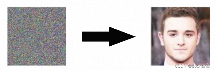
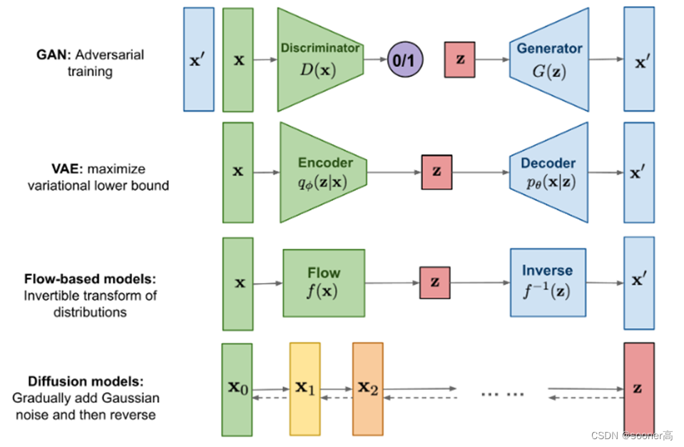
Diffusion Models work by destroying training data through the successive addition of Gaussian noise, and then learning to recover the data by reversing this noising process
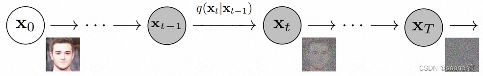
这个过程是通过逐渐的对输入数据(图像)加噪声,来获得最优的后验
q
(
x
1
:
T
∣
x
0
)
q(\mathbf{x}_{1:T}|\mathbf{x}_0)
q(x1:T∣x0),这里
x
1
,
.
.
.
,
x
T
\mathbf{x}_{1}, ..., \mathbf{x}_{T}
x1,...,xT是和
x
0
\mathbf{x}_0
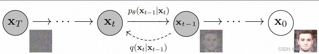
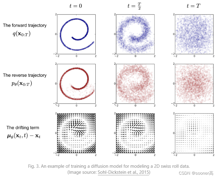
x0尺度一样的隐变量(latent variable),下图展示了这种加噪的过程: 最终,图像渐近变换为纯高斯噪声(pure Gaussian noise)。注意,我们训练扩散模型的目标,其实是学习反向过程:训练
p
θ
(
x
t
−
1
∣
x
t
)
p_{\theta}(\mathbf{x}_{t-1}|\mathbf{x}_{t})
pθ(xt−1∣xt),通过沿着这条马尔可夫链向后遍历,我们可以从噪声中恢复原始的图像:
训练效率方面高(✔ training efficiency): 扩散模型还具有可扩展性和并行性的额外好处, 因为其网络结构简单和训练规则清晰的原因,多机多卡的并行难度相比GAN来说低很多(GAN可能有很多级联的Generator和Discriminator,所以在设计并行训练时候通常需要进行一些复杂的手动切分模型操作)。
第1部分我们提到了Diffusion Model的目标: 训练
p
θ
(
x
t
−
1
∣
x
t
)
p_{\theta}(\mathbf{x}_{t-1}|\mathbf{x}_{t})
pθ(xt−1∣xt),通过沿着这条马尔可夫链向后遍历,我们可以从噪声中恢复原始的图像。
现在,我们需要一个数学上更正式的表达,因为最终需要一个可处理的损失函数,我们的神经网络需要优化它。
如上图(来自DDPM论文)所示,我们用
q
(
x
0
)
q(\mathbf{x_0})
q(x0)表示真实的训练数据分布(real images),我们可以从这个分布中任意采样得到图像:
x
0
∼
q
(
x
0
)
\mathbf{x_0} \sim q(\mathbf{x_0})
x0∼q(x0)。
3.1 Forward Pass 前向过程
q
(
x
t
∣
x
t
−
1
)
q(\mathbf{x}_t|\mathbf{x}_{t-1})
q(xt∣xt−1)
我们将前向过程(Forward pass, 在每个timestep上加Gaussian noise)
q
(
x
t
∣
x
t
−
1
)
q(\mathbf{x}_t|\mathbf{x}_{t-1})
q(xt∣xt−1), 根据已知的方差表
0
<
β
1
<
β
2
<
.
.
.
<
β
T
<
1
0 < \beta_1 < \beta_2 < ... < \beta_T < 1
0<β1<β2<...<βT<1,定义为:
q
(
x
t
∣
x
t
−
1
)
=
N
(
x
t
;
1
−
β
t
x
t
−
1
,
β
t
I
)
q(\mathbf{x}_t|\mathbf{x}_{t-1}) = \mathcal{N}(\mathbf{x}_t; \sqrt{1-\beta_t}\mathbf{x}_{t-1}, \beta_t\mathbf{I})
q(xt∣xt−1)=N(xt;1−βtxt−1,βtI)
我们知道,标准正态分布(
N
\mathcal{N}
N)由2个参数定义:
均值
μ
\mu
μ
标准差
σ
2
≥
0
\sigma^2 \ge0
σ2≥0
那么基本上,在时间步(timestep)
t
t
t上的新图像(slightly noisier new image)是从一个条件高斯分布(conditional Gaussian distribution) 中绘制的,其中
μ
t
=
1
−
β
t
x
t
−
1
,
σ
2
=
β
t
\mu_{t} = \sqrt{1-\beta_t}\mathbf{x}_{t-1}, \sigma^2=\beta_t
μt=1−βtxt−1,σ2=βt。
那这种情况下,时间步(timestep)
t
t
t上的新图像的生成过程,就可以转化为从标准正态分布中取的一个噪声 :
ϵ
∼
N
(
0
,
I
)
\epsilon \sim \mathcal{N}(0, \mathbf{I})
ϵ∼N(0,I),并让
x
t
=
1
−
β
t
x
t
−
1
+
β
t
ϵ
\mathbf{x}_t =\sqrt{1-\beta_t}\mathbf{x}_{t-1}+\sqrt{\beta_t}\epsilon
xt=1−βtxt−1+βtϵ
这里,
β
t
\beta_t
βt在每个timestep的值并不相同,事实上,
β
t
\beta_t
βt随timestep变化的过程可以理解为variance schedule,其变化可以是linear, quadratic, cosine的形式,类似于 学习率(learning rate) 的变化。
我理解这个
β
t
\beta_t
βt(either learned or fixed)的变化是研究人员根据任务收敛情况等内容设置的,此外,如果表现良好,当
T
T
T足够大的时候,
β
\beta
β的目标还是让Forward Pass中最后的
x
T
\mathbf{x}_T
xT变成一个pure/isotropic Gausssian noise[7]。
3.2 Backward Pass 后向过程
p
θ
(
x
t
−
1
∣
x
t
)
p_{\theta}(\mathbf{x}_{t-1}|\mathbf{x}_t)
pθ(xt−1∣xt)
刚刚Forward Pass解释完了,如果我们知道条件分布(conditional distribution)
p
(
x
t
−
1
∣
x
t
)
p(\mathbf{x}_{t-1}|\mathbf{x}_{t})
p(xt−1∣xt), 我们就可以进行Backward Process了:
即采样一些随机的Gaussian noise
x
T
\mathbf{x}_T
xT, 并逐渐的denoise它们,最终得到和真实数据分布一致的数据
x
0
\mathbf{x}_0
x0
但是,这个条件概率我们其实是不知道的,它很难处理(intractable),因为它需要知道所有可能图像的分布,以便计算这个条件概率。因此,我们想要利用神经网络的能力去approximate (learn) 这个条件概率 (conditional probability distribution)。
具体的,我们想要学习的条件概率的数学表达为
p
θ
(
x
t
−
1
∣
x
t
)
p_{\theta}(\mathbf{x}_{t-1}|\mathbf{x}_t)
pθ(xt−1∣xt), 其中
θ
\theta
θ代表了神经网络的参数,通过梯度进行优化。
所以我们将这个过程类比Forward Pass,进行如下表示:
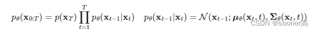
p
θ
(
x
t
−
1
∣
x
t
)
=
N
(
x
t
−
1
;
μ
θ
(
x
t
,
t
)
,
∑
θ
(
x
t
,
t
)
)
p_{\theta}(\mathbf{x}_{t-1}|\mathbf{x}_t) = \mathcal{N}(\mathbf{x}_{t-1};\mu_{\theta(\mathbf{x}_t, t)}, \sum_{\theta}(\mathbf{x}_t, t))
pθ(xt−1∣xt)=N(xt−1;μθ(xt,t),θ∑(xt,t))
根据论文所述,我们将上面的式子变成如下形式
p
θ
(
x
t
−
1
∣
x
t
)
=
N
(
x
t
−
1
;
μ
θ
(
x
t
,
t
)
,
σ
t
2
I
)
p_{\theta}(\mathbf{x}_{t-1}|\mathbf{x}_t) = \mathcal{N}(\mathbf{x}_{t-1};\mu_{\theta(\mathbf{x}_t, t)}, \sigma^2_{t}\mathbf{I})
pθ(xt−1∣xt)=N(xt−1;μθ(xt,t),σt2I)
为了获得Backward Pass中,均值
μ
θ
\mu_{\theta}
μθ的objective function(目标函数),Jonathon Ho等人观察到,
q
(
x
t
∣
x
t
−
1
)
q(\mathbf{x}_t|\mathbf{x}_{t-1})
q(xt∣xt−1)(Forward Pass)和
p
θ
(
x
t
−
1
∣
x
t
)
p_{\theta}(\mathbf{x}_{t-1}|\mathbf{x}_t)
pθ(xt−1∣xt)(Backward Pass)的组合可以视为一种VAE(Variational AutoEncoder)[8]。因此,根据VAE的概念,其变分下边界(variational lower bound, 也称为ELBO)[9]可以用于最小化相对于真实数据样本
x
0
\mathbf{x}_0
x0的负对数似然(negative log-likelihood)。
在这里,VAE的下界ELBO其实是每个timestep
t
t
t时的损失函数之和:
L
=
L
0
+
L
1
+
.
.
.
+
L
T
L=L_{0} + L_{1} + ... + L_{T}
L=L0+L1+...+LT。通过Forward Pass
q
(
x
t
∣
x
t
−
1
)
q(\mathbf{x}_t|\mathbf{x}_{t-1})
q(xt∣xt−1)和Backward Pass
p
θ
(
x
t
−
1
∣
x
t
)
p_{\theta}(\mathbf{x}_{t-1}|\mathbf{x}_t)
pθ(xt−1∣xt)的构建,损失函数
L
L
L的每一项, 除
L
0
L_0
L0以外,实际上就是2个Gaussian distributions的KL divergence (KL散度,用于衡量分布之间的相似性)。
像2015年ICML的论文Deep Unsupervised Learning using Nonequilibrium Thermodynamics[6]展示的那样,Forward Pass
q
(
x
t
∣
x
t
−
1
)
q(\mathbf{x}_t|\mathbf{x}_{t-1})
q(xt∣xt−1)构建的直接结果是我们可以在任意噪声水平(arbitrary noise level)下采样出
x
t
\mathbf{x}_t
xt(基于
x
0
\mathbf{x}_0
x0,因为高斯分布的和还是高斯分布, sums of Gaussians is also Gaussian)。这个思路很方便,这意味着我们可以直接从
x
0
\mathbf{x}_0
x0得到某个timestep
t
t
t时的
x
t
\mathbf{x}_t
xt, 而非迭代式的、线性的从
x
0
,
x
1
,
.
.
.
,
x
t
\mathbf{x}_0, \mathbf{x}_1, ..., \mathbf{x}_t
x0,x1,...,xt一步步的从
0
0
0走到
t
t
t,这种直接从
x
0
\mathbf{x}_0
x0到
x
t
\mathbf{x}_t
xt的方式用数学表达为如下形式:
q
(
x
t
∣
x
0
)
=
N
(
x
t
;
α
t
‾
x
0
,
(
1
−
α
t
‾
)
I
)
)
q(\mathbf{x}_t | \mathbf{x}_0) = \mathcal{N}(\mathbf{x}_t; \sqrt{\overline{\alpha_t}}\mathbf{x}_0, (1-\overline{\alpha_t})\mathbf{I}))
q(xt∣x0)=N(xt;αtx0,(1−αt)I))
这里,
q
(
x
t
∣
x
0
)
q(\mathbf{x}_t | \mathbf{x}_0)
q(xt∣x0)的推导过程如下:
其中,
α
t
:
=
1
−
β
t
,
α
t
‾
:
=
∏
s
=
1
t
α
s
\alpha_t := 1 - \beta_t, \overline{\alpha_t} := \prod_{s=1}^{t}\alpha_s
αt:=1−βt,αt:=∏s=1tαs, 我们把这个方程称为 “优雅的性质”(Nice property),这意味着我们可以对Gaussian noise进行采样并适当缩放, 从而可以直接地从
x
0
\mathbf{x}_0
x0得到
x
t
\mathbf{x}_t
xt。
这里需要注意的是,
α
t
‾
\overline{\alpha_t}
αt是已知的variance schedula
β
t
\beta_t
βt的函数,因此其是可以 预计算(precomputed) 的。这使得我们在训练过程中,可以随机的采样timestep
t
t
t,并优化对应的损失函数
L
t
L_t
Lt。
此外,如DDPM论文提到的那样(其中的数学解释的部分请参考What are Diffusion Models?这篇博客),其另一个优雅的性质是重新参数化平均值,使神经网络
ϵ
θ
(
x
t
,
t
)
\epsilon_{\theta}(\mathbf{x}_t, t)
ϵθ(xt,t)学习(预测)添加的噪声(Reparametrize the mean to make the neural network learn/predict the added noise (via a network
ϵ
θ
(
x
t
,
t
)
\epsilon_{\theta}(\mathbf{x}_t, t)
ϵθ(xt,t) for noise level
t
t
t)), 而这个添加的噪声就是loss function的KL term中的一项。
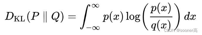
这里补充一下KL term,或者KL divergence的概念,其本质上就是衡量概率分布
P
P
P和概率分布
Q
Q
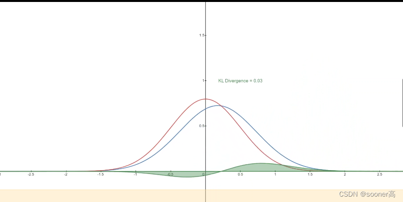
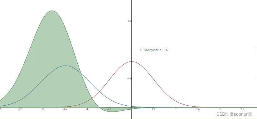
Q的距离的熵,是由Kullback和Leibler提出的一种相对熵的概念。 下图展示的是变化的分布P (blue) 和标准的正态部分Q (red)的KL 散度,绿色曲线表示上述KL散度定义中积分内的函数,可以看出,当P和Q越接近,KL Divergence的值就越小,反之则越来越大。
μ
θ
(
x
t
,
t
)
=
1
α
t
(
x
t
−
β
t
1
−
α
t
‾
ϵ
θ
(
x
t
,
t
)
)
\mu_{\theta}(\mathbf{x}_t, t) = \frac{1}{\sqrt{\alpha_t}} (\mathbf{x}_t - \frac{\beta_t}{\sqrt{1-\overline{\alpha_t}}}\epsilon_{\theta}(\mathbf{x}_t, t))
μθ(xt,t)=αt1(xt−1−αtβtϵθ(xt,t))
其推导过程如下
4.1
μ
θ
(
x
t
,
t
)
\mu_{\theta}(\mathbf{x}_t, t)
μθ(xt,t)的推导过程
回顾Backward Pass中的目标, 用
p
θ
(
x
t
−
1
∣
x
t
)
=
N
(
x
t
−
1
;
μ
θ
(
x
t
,
t
)
,
σ
t
2
I
)
p_{\theta}(\mathbf{x}_{t-1}|\mathbf{x}_t) = \mathcal{N}(\mathbf{x}_{t-1};\mu_{\theta(\mathbf{x}_t, t)}, \sigma^2_{t}\mathbf{I})
pθ(xt−1∣xt)=N(xt−1;μθ(xt,t),σt2I)来替代
q
(
x
t
−
1
∣
x
t
)
q(\mathbf{x}_{t-1}|\mathbf{x}_{t})
q(xt−1∣xt), 这是由于
q
(
x
t
−
1
∣
x
t
)
q(\mathbf{x}_{t-1}|\mathbf{x}_{t})
q(xt−1∣xt)的数据集很难用1个给定的先验数据分布来唯一确定,所以需要用一个神经网络
p
θ
p_{\theta}
pθ来学习 从Forward Pass的定义来看,虽然在逆向过程(reverse conditional probability)(
x
T
\mathbf{x}_T
xT到
x
0
\mathbf{x}_0
x0) 比较困难,但是当给定
x
0
\mathbf{x}_0
x0的时候,即当有
q
(
x
t
−
1
∣
x
t
,
x
0
)
q(\mathbf{x}_{t-1}|\mathbf{x}_{t},\mathbf{x}_{0})
q(xt−1∣xt,x0)的时候(先验多了真实数据
x
0
\mathbf{x}_0
x0), 此逆向过程可解:
4.2 目标/损失函数
由4.1可知,DDPM要优化的均值
μ
\mu
μ,经过了重参数化操作,变成了预测添加的噪声
ϵ
t
\epsilon_t
ϵt,最终,我们要优化的损失函数
L
t
L_t
Lt的表示如下:
∣
∣
ϵ
−
ϵ
θ
(
x
t
,
t
)
∣
∣
2
=
∣
∣
ϵ
−
ϵ
θ
(
α
t
‾
x
0
+
(
1
−
α
t
‾
)
ϵ
,
t
)
∣
∣
2
||\epsilon - \epsilon_{\theta}(\mathbf{x}_t, t) ||^2 = || \epsilon - \epsilon_{\theta}(\sqrt{\overline{\alpha_t}}\mathbf{x}_0 + \sqrt{(1-\overline{\alpha_t})}\epsilon, t) ||^2
∣∣ϵ−ϵθ(xt,t)∣∣2=∣∣ϵ−ϵθ(αtx0+(1−αt)ϵ,t)∣∣2
这里
x
0
\mathbf{x}_{0}
x0是原始的训练图片,
x
t
\mathbf{x}_{t}
xt是有固定的Forward pass在noise level
t
t
t得到的加噪结果。
ϵ
\epsilon
ϵ是在timestep
t
t
t采样得到的pure noise,
ϵ
θ
(
x
t
,
t
)
\epsilon_{\theta}(\mathbf{x}_t, t)
ϵθ(xt,t)则是我们的神经网络,其用一个简单的MSE Loss来优化真实的Gaussian noise和预测的Gaussian noise。
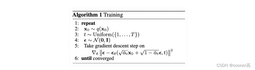
训练代码解释如下(最通俗解释):
① 从训练集随机采样一个原始数据
x
0
\mathbf{x}_{0}
x0
② 从
0
到
T
0 到 T
0到T中间,随机选取一个timestep
t
t
t, 可以直接通过
q
(
x
t
∣
x
0
)
q(\mathbf{x}_t | \mathbf{x}_0)
q(xt∣x0)获得
x
t
\mathbf{x}_t
xt,
x
t
\mathbf{x}_t
xt即为对原始数据
x
0
\mathbf{x}_{0}
x0的加噪的结构(或者说是corrupted result)
③ 随机从
N
(
0
,
I
)
\mathcal{N}(0, \mathbf{I})
N(0,I)采样得到噪声
ϵ
\epsilon
ϵ
④ 将 timestep
t
t
t, 系数
α
t
‾
:
=
∏
s
=
1
t
α
s
\overline{\alpha_t} := \prod_{s=1}^{t}\alpha_s
αt:=∏s=1tαs, 图片数据
x
0
\mathbf{x}_{0}
x0和 Gaussian noise
ϵ
\epsilon
ϵ输入到神经网络
ϵ
θ
\epsilon_{\theta}
ϵθ中,得到预测值,然后让其和真实的采样得到的噪声
ϵ
\epsilon
ϵ进行MSE Loss,用来优化神经网络
ϵ
θ
\epsilon_{\theta}
ϵθ
classAttention(nn.Module):def__init__(self, dim, heads=4, dim_head=32):super().__init__()
self.scale = dim_head**-0.5
self.heads = heads
hidden_dim = dim_head * heads
self.to_qkv = nn.Conv2d(dim, hidden_dim *3,1, bias=False)
self.to_out = nn.Conv2d(hidden_dim, dim,1)defforward(self, x):
b, c, h, w = x.shape
qkv = self.to_qkv(x).chunk(3, dim=1)
q, k, v =map(lambda t: rearrange(t,"b (h c) x y -> b h c (x y)", h=self.heads), qkv
)
q = q * self.scale
sim = einsum("b h d i, b h d j -> b h i j", q, k)
sim = sim - sim.amax(dim=-1, keepdim=True).detach()
attn = sim.softmax(dim=-1)
out = einsum("b h i j, b h d j -> b h i d", attn, v)
out = rearrange(out,"b h (x y) d -> b (h d) x y", x=h, y=w)return self.to_out(out)classLinearAttention(nn.Module):def__init__(self, dim, heads=4, dim_head=32):super().__init__()
self.scale = dim_head**-0.5
self.heads = heads
hidden_dim = dim_head * heads
self.to_qkv = nn.Conv2d(dim, hidden_dim *3,1, bias=False)
self.to_out = nn.Sequential(nn.Conv2d(hidden_dim, dim,1),
nn.GroupNorm(1, dim))defforward(self, x):
b, c, h, w = x.shape
qkv = self.to_qkv(x).chunk(3, dim=1)
q, k, v =map(lambda t: rearrange(t,"b (h c) x y -> b h c (x y)", h=self.heads), qkv
)
q = q.softmax(dim=-2)
k = k.softmax(dim=-1)
q = q * self.scale
context = torch.einsum("b h d n, b h e n -> b h d e", k, v)
out = torch.einsum("b h d e, b h d n -> b h e n", context, q)
out = rearrange(out,"b h c (x y) -> b (h c) x y", h=self.heads, x=h, y=w)return self.to_out(out)
Sinusoidal time embeddings (timestep embedding 的目的是告知模型,输入对应的noise level
t
t
t, 也可理解成输入在Markov chain中的位置, 和NeRF中的positional encoding的意义差不多。)
from datasets import load_dataset
# load dataset from the hub
dataset = load_dataset("fashion_mnist")
image_size =28
channels =1
batch_size =128from torchvision import transforms
from torch.utils.data import DataLoader
# define image transformations (e.g. using torchvision)
transform = Compose([
transforms.RandomHorizontalFlip(),
transforms.ToTensor(),
transforms.Lambda(lambda t:(t *2)-1)])# define functiondeftransforms(examples):
examples["pixel_values"]=[transform(image.convert("L"))for image in examples["image"]]del examples["image"]return examples
transformed_dataset = dataset.with_transform(transforms).remove_columns("label")# create dataloader
dataloader = DataLoader(transformed_dataset["train"], batch_size=batch_size, shuffle=True)
Ok, 数据加载器Dataloader完成后,还需要进行Sampling的定义,从而能验证噪声预测器模型
ϵ
θ
\epsilon_{\theta}
ϵθ训练的效果(即从
x
T
→
x
0
\mathbf{x}_T \rightarrow \mathbf{x}_0
xT→x0),采样Sampling的逻辑定义如下: 从扩散模型生成新图像是通过逆转扩散过程来实现的:从
T
T
T开始,从 纯粹的高斯分布(Gaussian distribution) 中采样噪声, 然后使用我们的神经网络逐渐去噪(使用网络学到的条件概率),然后到
t
=
0
t=0
t=0结束。显然,我们可以通过插入重参数化的均值,使用我们的噪声预测器
ϵ
θ
\epsilon_{\theta}
ϵθ,得到去噪后的图像
x
t
−
1
\mathbf{x}_{t-1}
xt−1。
注意:DDPM的variance是fix的,所以这里不需要考虑variance(方差)的影响。
理想情况下,我们最终得到的图像看起来像是来自真实的数据分布, 其代码如下:
@torch.no_grad()defp_sample(model, x, t, t_index):
betas_t = extract(betas, t, x.shape)
sqrt_one_minus_alphas_cumprod_t = extract(
sqrt_one_minus_alphas_cumprod, t, x.shape
)
sqrt_recip_alphas_t = extract(sqrt_recip_alphas, t, x.shape)# Equation 11 in the paper# Use our model (noise predictor) to predict the mean
model_mean = sqrt_recip_alphas_t *(
x - betas_t * model(x, t)/ sqrt_one_minus_alphas_cumprod_t
)if t_index ==0:return model_mean
else:
posterior_variance_t = extract(posterior_variance, t, x.shape)
noise = torch.randn_like(x)# Algorithm 2 line 4:return model_mean + torch.sqrt(posterior_variance_t)* noise
# Algorithm 2 (including returning all images)@torch.no_grad()defp_sample_loop(model, shape):
device =next(model.parameters()).device
b = shape[0]# start from pure noise (for each example in the batch)
img = torch.randn(shape, device=device)
imgs =[]for i in tqdm(reversed(range(0, timesteps)), desc='sampling loop time step', total=timesteps):
img = p_sample(model, img, torch.full((b,), i, device=device, dtype=torch.long), i)
imgs.append(img.cpu().numpy())return imgs
@torch.no_grad()defsample(model, image_size, batch_size=16, channels=3):return p_sample_loop(model, shape=(batch_size, channels, image_size, image_size))
当模型训练完毕后,我们将随机从Gaussian Distribution中采样得到
x
T
\mathbf{x}_T
xT, 然后通过reverse/backward diffusion process得到其对应的
x
0
\mathbf{x}_0
x0,代码就是6.3中的Sampling,其结果如下(图像分辨率是
28
×
28
28 \times 28
28×28):
# sample 64 images
samples = sample(model, image_size=image_size, batch_size=64, channels=channels)# show a random one
random_index =5
plt.imshow(samples[-1][random_index].reshape(image_size, image_size, channels), cmap="gray")